3  Morphological Processing, Connected Components, and Segmentation

3.1 Introduction to Mathematical Morphology

Morphological image processing is a collection of techniques that extract and transform image features based on their geometric and topological properties. Unlike filtering operations that modify pixel intensities directly, morphological operations modify the structure and shape of objects in binary and grayscale images. These operations are rooted in mathematical morphology, which uses set theory as its foundational language.

When working with images, we represent objects as sets of pixels. In a binary image, foreground pixels (typically white or valued 1) represent objects of interest, and background pixels (typically black or valued 0) constitute the complement. The power of morphological operations lies in their ability to extract meaningful structural information—identifying boundaries, separating touching objects, removing noise, and filling gaps—while operating on simple local neighborhood rules.

3.1.1 Core Concept: The Structuring Element

All morphological operations pivot on the structuring element (SE), a small binary template that defines the neighborhood pattern considered during processing. Think of the structuring element as a shape stamp that we place on every pixel of the image. Depending on where this stamp fits relative to the foreground, we make decisions about whether to keep, add, or remove that pixel.

The structuring element specifies: 1. Which neighboring pixels to consider through its spatial extent and shape 2. The decision logic for whether the center pixel becomes foreground or background 3. The relative importance of different neighbors through its geometry

Common structuring element shapes include disks (circular approximations), squares, crosses, and diamonds. The choice of shape and size fundamentally determines which features are enhanced or suppressed.

3.2 Binary Morphological Operations

3.2.1 Erosion: Shrinking Foreground Regions

Intuitive Explanation:

Erosion shrinks white (foreground) regions. Imagine placing the structuring element on every part of the image. For a pixel to become (or remain) white in the eroded result, the entire structuring element must fit completely inside the white region when centered on that pixel. If any part of the structuring element overlaps black (background), that pixel becomes black.

Key Effects:

  • Thins and shrinks foreground objects
  • Removes small isolated foreground pixels entirely
  • Breaks narrow connections between objects
  • Enlarges background regions (equivalently, shrinks foreground)

When to Use:

  • Removing noise (small white speckles disappear)
  • Separating touching objects
  • Extracting the “skeleton” or core of objects
  • Pre-processing for feature extraction

3.2.2 Dilation: Expanding Foreground Regions

Intuitive Explanation:

Dilation expands white (foreground) regions. A pixel becomes white in the dilated result if any part of the structuring element overlaps foreground pixels when centered on that position. This has the effect of “growing” or “fattening” the foreground.

Key Effects:

  • Thickens and expands foreground objects
  • Fills small black holes inside foreground regions
  • Closes narrow gaps between foreground regions
  • Shrinks background regions

When to Use:

  • Filling holes in segmented objects
  • Connecting nearly-touching components
  • Recovering partially eroded structures
  • Smoothing rough object boundaries

3.2.3 Opening: Erosion Followed by Dilation

Effect:

Opening removes small foreground objects and noise while attempting to preserve the size and shape of larger objects. The erosion step removes small components; the subsequent dilation restores much of the original size of remaining components.

Key Property: Opening is idempotent—applying it multiple times produces the same result as applying it once.

When to Use:

  • Removing small noise pixels without destroying main features
  • Separating nearby objects before counting
  • Pre-processing binary masks before analysis
  • Cleaning segmentation results

3.2.4 Closing: Dilation Followed by Erosion

Effect:

Closing fills small holes inside foreground regions while attempting to preserve the overall size. The dilation step fills gaps and holes; the subsequent erosion attempts to restore the original boundary.

Key Property: Closing is also idempotent.

When to Use:

  • Filling gaps inside nuclei or cells
  • Smoothing object interiors
  • Bridging narrow gaps in incomplete contours
  • Consolidating fragmented regions

3.3 Practical Implementation: Morphological Operations on Test Image

Let us demonstrate all four fundamental operations on a carefully constructed test image. This image contains a central rounded region with intentional imperfections: a small noise pixel, a small hole, and subtle boundary irregularities.

import numpy as np
import matplotlib.pyplot as plt
from skimage import morphology
import matplotlib.patches as patches

# Create test image with known structure
image = np.array([
    [1.0, 1.0, 1.0, 1.0, 1.0, 1.0, 1.0, 1.0, 1.0, 1.0],
    [1.0, 0.8, 0.8, 0.8, 0.8, 0.8, 0.8, 0.8, 0.5, 1.0],
    [1.0, 0.8, 0.6, 0.6, 0.6, 0.6, 0.6, 0.6, 0.8, 1.0],
    [1.0, 0.8, 0.6, 0.4, 0.4, 0.4, 0.4, 0.6, 0.8, 1.0],
    [1.0, 0.8, 0.6, 0.4, 1.0, 0.1, 0.4, 0.6, 0.8, 1.0],  # Hole at (4,4), noise at (4,4)
    [1.0, 0.8, 0.6, 0.4, 0.0, 0.0, 0.4, 0.6, 0.8, 1.0],
    [1.0, 0.8, 0.6, 0.4, 0.4, 0.4, 0.4, 0.6, 0.8, 1.0],
    [1.0, 0.8, 0.6, 0.6, 0.6, 0.6, 0.6, 0.5, 0.8, 1.0],
    [1.0, 0.8, 0.8, 0.8, 0.8, 0.8, 0.8, 0.8, 0.8, 1.0],
    [1.0, 1.0, 1.0, 1.0, 1.0, 1.0, 1.0, 1.0, 1.0, 1.0]
], dtype=np.float32)

# Display the original image with annotations
fig, ax = plt.subplots(1, 1, figsize=(6, 6))
ax.imshow(image, cmap='gray', interpolation='nearest', vmin=0, vmax=1)
ax.set_title("Original Test Image\n(Contains hole and noise)", fontsize=12, fontweight='bold')
ax.grid(True, alpha=0.3)
ax.set_xticks(range(10))
ax.set_yticks(range(10))

# Annotate features
ax.plot(8, 1, 'r*', markersize=15, label='Noise pixel (boundary roughness)')
ax.plot(4, 4, 'b*', markersize=15, label='Hole')
ax.legend(loc='upper left', fontsize=9)
plt.tight_layout()
plt.show()

print("Original image shape:", image.shape)
print("Foreground pixels in original:", np.sum(image > 0.5))

Original image shape: (10, 10)
Foreground pixels in original: 83

3.3.1 Structuring Elements

The structuring element defines the locality of each operation. We demonstrate with a disk-shaped structuring element, which is rotationally symmetric and commonly used in medical image analysis.

# Create structuring elements of different sizes
selem_1 = morphology.disk(1)
selem_2 = morphology.disk(2)

print("Disk structuring element (radius 1):")
print(selem_1.astype(int))
print("\nDisk structuring element (radius 2):")
print(selem_2.astype(int))

# Visualize the structuring elements
fig, axes = plt.subplots(1, 2, figsize=(8, 4))

axes[0].imshow(selem_1.astype(int), cmap='gray', interpolation='nearest')
axes[0].set_title("Disk SE (radius=1)", fontsize=11)
axes[0].grid(True, alpha=0.3)
axes[0].set_xticks(range(selem_1.shape[1]))
axes[0].set_yticks(range(selem_1.shape[0]))

axes[1].imshow(selem_2.astype(int), cmap='gray', interpolation='nearest')
axes[1].set_title("Disk SE (radius=2)", fontsize=11)
axes[1].grid(True, alpha=0.3)
axes[1].set_xticks(range(selem_2.shape[1]))
axes[1].set_yticks(range(selem_2.shape[0]))

plt.tight_layout()
plt.show()

print("\nStructuring element as binary: 1 = included, 0 = excluded")
Disk structuring element (radius 1):
[[0 1 0]
 [1 1 1]
 [0 1 0]]

Disk structuring element (radius 2):
[[0 0 1 0 0]
 [0 1 1 1 0]
 [1 1 1 1 1]
 [0 1 1 1 0]
 [0 0 1 0 0]]


Structuring element as binary: 1 = included, 0 = excluded

3.3.2 Converting to Binary and Applying Operations

For morphological operations in scikit-image, we work with binary (uint8) images. The convention is white (255) = foreground and black (0) = background.

# Convert floating-point image to binary uint8
# Threshold: pixels > 0.5 become foreground
binary_image = (image > 0.5).astype(np.uint8) * 255

print("Binary image (thresholded at 0.5):")
print(binary_image)
print("\nForeground pixels:", np.sum(binary_image > 0))

# Apply morphological operations with radius-1 disk
selem = morphology.disk(1)

eroded = morphology.erosion(binary_image, selem)
dilated = morphology.dilation(binary_image, selem)
opened = morphology.opening(binary_image, selem)
closed = morphology.closing(binary_image, selem)

# Convert back to [0, 1] for visualization
eroded_float = eroded.astype(np.float32) / 255.0
dilated_float = dilated.astype(np.float32) / 255.0
opened_float = opened.astype(np.float32) / 255.0
closed_float = closed.astype(np.float32) / 255.0

print("\nForeground pixels after operations:")
print(f"  Original:  {np.sum(binary_image > 0)}")
print(f"  Erosion:   {np.sum(eroded > 0)}")
print(f"  Dilation:  {np.sum(dilated > 0)}")
print(f"  Opening:   {np.sum(opened > 0)}")
print(f"  Closing:   {np.sum(closed > 0)}")
Binary image (thresholded at 0.5):
[[255 255 255 255 255 255 255 255 255 255]
 [255 255 255 255 255 255 255 255   0 255]
 [255 255 255 255 255 255 255 255 255 255]
 [255 255 255   0   0   0   0 255 255 255]
 [255 255 255   0 255   0   0 255 255 255]
 [255 255 255   0   0   0   0 255 255 255]
 [255 255 255   0   0   0   0 255 255 255]
 [255 255 255 255 255 255 255   0 255 255]
 [255 255 255 255 255 255 255 255 255 255]
 [255 255 255 255 255 255 255 255 255 255]]

Foreground pixels: 83

Foreground pixels after operations:
  Original:  83
  Erosion:   60
  Dilation:  99
  Opening:   82
  Closing:   95

3.3.3 Visualizing All Operations

# Create comprehensive visualization
fig, axes = plt.subplots(2, 3, figsize=(16, 10))

# Original (converted to binary for comparison)
axes[0, 0].imshow(binary_image / 255.0, cmap='gray', interpolation='nearest', vmin=0, vmax=1)
axes[0, 0].set_title("Original Binary Image", fontsize=12, fontweight='bold')
axes[0, 0].grid(True, alpha=0.3)
axes[0, 0].set_xticks(range(10))
axes[0, 0].set_yticks(range(10))

# Erosion
axes[0, 1].imshow(eroded_float, cmap='gray', interpolation='nearest', vmin=0, vmax=1)
axes[0, 1].set_title("Erosion (shrinks foreground)", fontsize=12, fontweight='bold')
axes[0, 1].grid(True, alpha=0.3)
axes[0, 1].set_xticks(range(10))
axes[0, 1].set_yticks(range(10))

# Dilation
axes[0, 2].imshow(dilated_float, cmap='gray', interpolation='nearest', vmin=0, vmax=1)
axes[0, 2].set_title("Dilation (expands foreground)", fontsize=12, fontweight='bold')
axes[0, 2].grid(True, alpha=0.3)
axes[0, 2].set_xticks(range(10))
axes[0, 2].set_yticks(range(10))

# Opening
axes[1, 0].imshow(opened_float, cmap='gray', interpolation='nearest', vmin=0, vmax=1)
axes[1, 0].set_title("Opening (erode → dilate)\nRemoves noise", fontsize=12, fontweight='bold')
axes[1, 0].grid(True, alpha=0.3)
axes[1, 0].set_xticks(range(10))
axes[1, 0].set_yticks(range(10))

# Closing
axes[1, 1].imshow(closed_float, cmap='gray', interpolation='nearest', vmin=0, vmax=1)
axes[1, 1].set_title("Closing (dilate → erode)\nFills holes", fontsize=12, fontweight='bold')
axes[1, 1].grid(True, alpha=0.3)
axes[1, 1].set_xticks(range(10))
axes[1, 1].set_yticks(range(10))

# Comparison: Open then Close
open_then_close = morphology.closing(opened, selem)
axes[1, 2].imshow(open_then_close.astype(np.float32) / 255.0, cmap='gray', 
                   interpolation='nearest', vmin=0, vmax=1)
axes[1, 2].set_title("Opening → Closing\nClean segmentation", fontsize=12, fontweight='bold')
axes[1, 2].grid(True, alpha=0.3)
axes[1, 2].set_xticks(range(10))
axes[1, 2].set_yticks(range(10))

plt.tight_layout()
plt.show()

3.4 Practical Demonstration: All Four Operations on Grayscale Image

We now apply all four morphological operations to a realistic test image that mimics a biological structure (like a nucleus surrounded by cytoplasm). The image has multiple intensity levels rather than being purely binary, demonstrating how morphological operations work on continuous-valued data.

import numpy as np
import matplotlib.pyplot as plt
from skimage import morphology

# Create a 10x10 grayscale image with a nucleus-like structure
# Outer ring (white) represents cytoplasm
# Inner region (gray to dark) represents nucleus with internal features
image = np.array([
    [1.0, 1.0, 1.0, 1.0, 1.0, 1.0, 1.0, 1.0, 1.0, 1.0],
    [1.0, 0.8, 0.8, 0.8, 0.8, 0.8, 0.8, 0.8, 0.5, 1.0],
    [1.0, 0.8, 0.6, 0.6, 0.6, 0.6, 0.6, 0.6, 0.8, 1.0],
    [1.0, 0.8, 0.6, 0.4, 0.4, 0.4, 0.4, 0.6, 0.8, 1.0],
    [1.0, 0.8, 0.6, 0.4, 1.0, 0.1, 0.4, 0.6, 0.8, 1.0],
    [1.0, 0.8, 0.6, 0.4, 0.0, 0.0, 0.4, 0.6, 0.8, 1.0],
    [1.0, 0.8, 0.6, 0.4, 0.4, 0.4, 0.4, 0.6, 0.8, 1.0],
    [1.0, 0.8, 0.6, 0.6, 0.6, 0.6, 0.6, 0.5, 0.8, 1.0],
    [1.0, 0.8, 0.8, 0.8, 0.8, 0.8, 0.8, 0.8, 0.8, 1.0],
    [1.0, 1.0, 1.0, 1.0, 1.0, 1.0, 1.0, 1.0, 1.0, 1.0]
], dtype=np.float32)

# Convert to uint8 for morphology operations
# Range: 0 (black) to 255 (white)
binary_uint8 = (image * 255).astype(np.uint8)

print("Original image (float scale [0,1]):")
print(image)
print("\nConverted to uint8 [0,255]:")
print(binary_uint8)

# Create structuring element (disk with radius 1)
selem = morphology.disk(1)

# Apply all four fundamental morphological operations
eroded = morphology.erosion(binary_uint8, selem)
dilated = morphology.dilation(binary_uint8, selem)
opened = morphology.opening(binary_uint8, selem)
closed = morphology.closing(binary_uint8, selem)

print("\nMorphological operation descriptions:")
print("  Erosion:  shrinks white regions")
print("  Dilation: expands white regions")
print("  Opening:  erosion then dilation (removes small objects)")
print("  Closing:  dilation then erosion (fills small holes)")

# Convert back to float [0,1] for display
eroded = eroded.astype(np.float32) / 255.0
dilated = dilated.astype(np.float32) / 255.0
opened = opened.astype(np.float32) / 255.0
closed = closed.astype(np.float32) / 255.0

# Visualize all operations
fig, axes = plt.subplots(2, 3, figsize=(15, 10))

axes[0, 0].imshow(image, cmap='gray', interpolation='nearest', vmin=0, vmax=1)
axes[0, 0].set_title("Original Grayscale Image", fontsize=12, fontweight='bold')
axes[0, 0].grid(True, alpha=0.3)
axes[0, 0].set_xticks(range(10))
axes[0, 0].set_yticks(range(10))

axes[0, 1].imshow(eroded, cmap='gray', interpolation='nearest', vmin=0, vmax=1)
axes[0, 1].set_title("Erosion", fontsize=12, fontweight='bold')
axes[0, 1].grid(True, alpha=0.3)
axes[0, 1].set_xticks(range(10))
axes[0, 1].set_yticks(range(10))

axes[0, 2].imshow(dilated, cmap='gray', interpolation='nearest', vmin=0, vmax=1)
axes[0, 2].set_title("Dilation", fontsize=12, fontweight='bold')
axes[0, 2].grid(True, alpha=0.3)
axes[0, 2].set_xticks(range(10))
axes[0, 2].set_yticks(range(10))

axes[1, 0].imshow(opened, cmap='gray', interpolation='nearest', vmin=0, vmax=1)
axes[1, 0].set_title("Opening", fontsize=12, fontweight='bold')
axes[1, 0].grid(True, alpha=0.3)
axes[1, 0].set_xticks(range(10))
axes[1, 0].set_yticks(range(10))

axes[1, 1].imshow(closed, cmap='gray', interpolation='nearest', vmin=0, vmax=1)
axes[1, 1].set_title("Closing", fontsize=12, fontweight='bold')
axes[1, 1].grid(True, alpha=0.3)
axes[1, 1].set_xticks(range(10))
axes[1, 1].set_yticks(range(10))

axes[1, 2].axis('off')

plt.tight_layout()
plt.show()
Original image (float scale [0,1]):
[[1.  1.  1.  1.  1.  1.  1.  1.  1.  1. ]
 [1.  0.8 0.8 0.8 0.8 0.8 0.8 0.8 0.5 1. ]
 [1.  0.8 0.6 0.6 0.6 0.6 0.6 0.6 0.8 1. ]
 [1.  0.8 0.6 0.4 0.4 0.4 0.4 0.6 0.8 1. ]
 [1.  0.8 0.6 0.4 1.  0.1 0.4 0.6 0.8 1. ]
 [1.  0.8 0.6 0.4 0.  0.  0.4 0.6 0.8 1. ]
 [1.  0.8 0.6 0.4 0.4 0.4 0.4 0.6 0.8 1. ]
 [1.  0.8 0.6 0.6 0.6 0.6 0.6 0.5 0.8 1. ]
 [1.  0.8 0.8 0.8 0.8 0.8 0.8 0.8 0.8 1. ]
 [1.  1.  1.  1.  1.  1.  1.  1.  1.  1. ]]

Converted to uint8 [0,255]:
[[255 255 255 255 255 255 255 255 255 255]
 [255 204 204 204 204 204 204 204 127 255]
 [255 204 153 153 153 153 153 153 204 255]
 [255 204 153 102 102 102 102 153 204 255]
 [255 204 153 102 255  25 102 153 204 255]
 [255 204 153 102   0   0 102 153 204 255]
 [255 204 153 102 102 102 102 153 204 255]
 [255 204 153 153 153 153 153 127 204 255]
 [255 204 204 204 204 204 204 204 204 255]
 [255 255 255 255 255 255 255 255 255 255]]

Morphological operation descriptions:
  Erosion:  shrinks white regions
  Dilation: expands white regions
  Opening:  erosion then dilation (removes small objects)
  Closing:  dilation then erosion (fills small holes)

3.5 Edge Detection with Sobel Filtering

3.5.1 Mathematical Foundation: Partial Derivatives and Gradients

Edge detection at its core is about identifying regions in an image where intensity changes rapidly. Mathematically, this is captured by computing derivatives with respect to spatial coordinates. For a continuous 2D function \(I(x, y)\) representing image intensity, the gradient is a vector composed of partial derivatives in the \(x\) and \(y\) directions:

\[\nabla I = \left( \frac{\partial I}{\partial x}, \frac{\partial I}{\partial y} \right)\]

The magnitude of the gradient indicates the strength of intensity change:

\[|\nabla I| = \sqrt{\left(\frac{\partial I}{\partial x}\right)^2 + \left(\frac{\partial I}{\partial y}\right)^2}\]

High gradient magnitudes occur at edges—regions where intensity transitions sharply from one level to another. In discrete digital images, we approximate these partial derivatives using finite differences computed with small convolution kernels.

3.5.2 The Sobel Operator: Discrete Approximation

The Sobel operator, developed by Irwin Sobel in the 1960s for use in computer vision and image processing, provides an efficient method for computing approximate derivatives using small \(3 \times 3\) kernels. Sobel’s innovation was to weight the central row/column more heavily than the edges, reducing noise sensitivity while approximating derivatives.

The Sobel operator consists of two kernels, \(S_x\) and \(S_y\), designed to approximate the partial derivatives in the \(x\) and \(y\) directions respectively:

Sobel kernel for \(x\)-direction (\(S_x\), detecting vertical edges):

\[S_x = \begin{bmatrix} -1 & 0 & +1 \\ -2 & 0 & +2 \\ -1 & 0 & +1 \end{bmatrix}\]

Sobel kernel for \(y\)-direction (\(S_y\), detecting horizontal edges):

\[S_y = \begin{bmatrix} -1 & -2 & -1 \\ 0 & 0 & 0 \\ +1 & +2 & +1 \end{bmatrix}\]

Note that \(S_y\) is the transpose of \(S_x\). The center element is always zero, and the weights along the center row/column are doubled (±2 instead of ±1) to emphasize central differences.

3.5.3 How Sobel Works: Convolution Process

For each pixel \((i, j)\) in the image, the Sobel operator:

  1. Extracts the \(3 \times 3\) neighborhood centered at \((i, j)\)
  2. Applies \(S_x\) convolution to compute \(\frac{\partial I}{\partial x}\), yielding a gradient estimate in the \(x\)-direction
  3. Applies \(S_y\) convolution to compute \(\frac{\partial I}{\partial y}\), yielding a gradient estimate in the \(y\)-direction
  4. Computes the gradient magnitude: \(|\nabla I| = \sqrt{G_x^2 + G_y^2}\)
  5. Assigns this magnitude to the output at position \((i, j)\)

Pixels with high gradient magnitude correspond to edges; pixels with low gradient magnitude correspond to smooth, uniform regions.

3.5.4 Sobel’s Contribution to Computer Vision

Irwin Sobel, working at Stanford University in the 1960s, developed this operator as part of early research in automated image analysis. His key insight was that a weighted averaging scheme—heavier weight on central differences—could produce robust edge detection even with camera noise and image degradation. The Sobel operator has become one of the most widely used edge detection methods, often serving as a baseline for more sophisticated approaches. Its simplicity, computational efficiency, and effectiveness have ensured its continued use across decades of computer vision applications, from autonomous vehicles to medical imaging.

3.5.5 Practical Application: Nucleus-Cytoplasm Boundary Detection

We now demonstrate Sobel edge detection on a synthetic image resembling a cell nucleus (darker region) surrounded by cytoplasm (lighter region). This mimics typical scenarios in biomedical image analysis where identifying cellular boundaries is critical.

import numpy as np
import matplotlib.pyplot as plt
from scipy import signal

# Create synthetic image: nucleus (low intensity) surrounded by cytoplasm (high intensity)
# White 2-pixel border represents the image background/boundary
nucleus_cytoplasm = np.array([
    [1.0, 1.0, 1.0, 1.0, 1.0, 1.0, 1.0, 1.0, 1.0, 1.0],
    [1.0, 1.0, 1.0, 1.0, 1.0, 1.0, 1.0, 1.0, 1.0, 1.0],
    [1.0, 1.0, 0.4, 0.4, 0.4, 0.4, 0.4, 0.4, 1.0, 1.0],
    [1.0, 1.0, 0.4, 0.2, 0.2, 0.2, 0.2, 0.4, 1.0, 1.0],
    [1.0, 1.0, 0.4, 0.2, 0.2, 0.2, 0.2, 0.4, 1.0, 1.0],
    [1.0, 1.0, 0.4, 0.2, 0.2, 0.2, 0.2, 0.4, 1.0, 1.0],
    [1.0, 1.0, 0.4, 0.2, 0.2, 0.2, 0.2, 0.4, 1.0, 1.0],
    [1.0, 1.0, 0.4, 0.4, 0.4, 0.4, 0.4, 0.4, 1.0, 1.0],
    [1.0, 1.0, 1.0, 1.0, 1.0, 1.0, 1.0, 1.0, 1.0, 1.0],
    [1.0, 1.0, 1.0, 1.0, 1.0, 1.0, 1.0, 1.0, 1.0, 1.0]
], dtype=np.float32)

print("Original image (nucleus with white 2-pixel border):")
print(nucleus_cytoplasm)

# Define Sobel kernels
S_x = np.array([
    [-1, 0, +1],
    [-2, 0, +2],
    [-1, 0, +1]
], dtype=np.float32)

S_y = np.array([
    [-1, -2, -1],
    [0, 0, 0],
    [+1, +2, +1]
], dtype=np.float32)

print("\nSobel kernel for x-direction (S_x) - vertical edge detection:")
print(S_x)

print("\nSobel kernel for y-direction (S_y) - horizontal edge detection:")
print(S_y)

# Apply Sobel using correlate2d (standard Sobel without kernel flipping)
# Note: scipy.signal.correlate2d does NOT flip the kernel (unlike ndimage.convolve)
# This matches the standard Sobel implementation in skimage.filters.sobel()
G_x = signal.correlate2d(nucleus_cytoplasm, S_x, mode='same', boundary='fill', fillvalue=0.0)
G_y = signal.correlate2d(nucleus_cytoplasm, S_y, mode='same', boundary='fill', fillvalue=0.0)

# Compute gradient magnitude
G_magnitude = np.sqrt(G_x**2 + G_y**2)

# Compute gradient angle (for reference)
G_angle = np.arctan2(G_y, G_x)

print("\nGradient in x-direction (G_x) - vertical edge detection:")
print(np.around(G_x, decimals=2))

print("\nGradient in y-direction (G_y) - horizontal edge detection:")
print(np.around(G_y, decimals=2))

print("\nGradient magnitude (edges highlighted):")
print(np.around(G_magnitude, decimals=2))

# Visualize
fig, axes = plt.subplots(2, 3, figsize=(16, 10))

# Original image
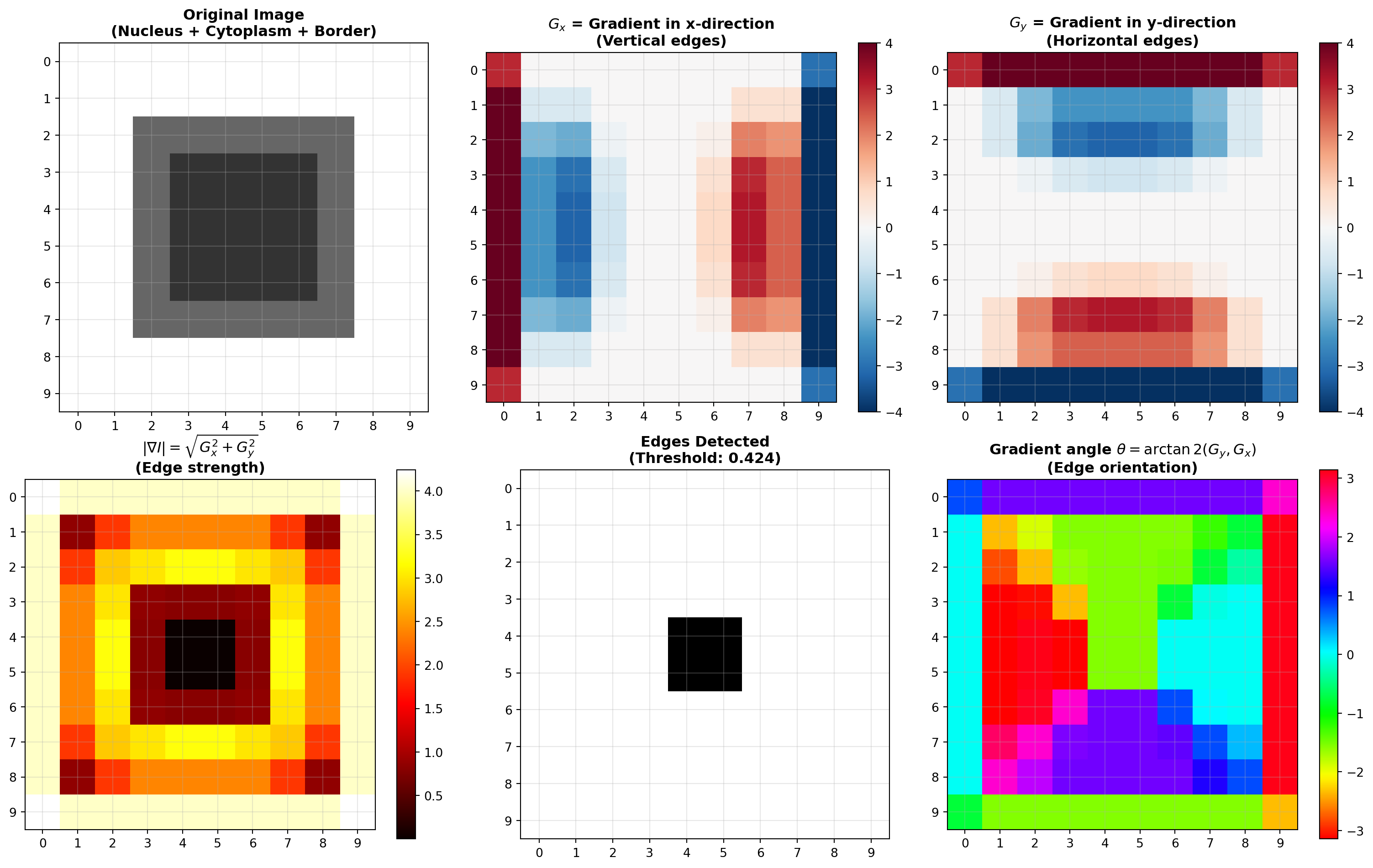
axes[0, 0].imshow(nucleus_cytoplasm, cmap='gray', interpolation='nearest', vmin=0, vmax=1)
axes[0, 0].set_title("Original Image\n(Nucleus + Cytoplasm + Border)", fontsize=12, fontweight='bold')
axes[0, 0].grid(True, alpha=0.3)
axes[0, 0].set_xticks(range(10))
axes[0, 0].set_yticks(range(10))

# Gradient in x-direction
im_gx = axes[0, 1].imshow(G_x, cmap='RdBu_r', interpolation='nearest')
axes[0, 1].set_title(r"$G_x$ = Gradient in x-direction" + "\n(Vertical edges)", fontsize=12, fontweight='bold')
axes[0, 1].grid(True, alpha=0.3)
axes[0, 1].set_xticks(range(10))
axes[0, 1].set_yticks(range(10))
plt.colorbar(im_gx, ax=axes[0, 1])

# Gradient in y-direction
im_gy = axes[0, 2].imshow(G_y, cmap='RdBu_r', interpolation='nearest')
axes[0, 2].set_title(r"$G_y$ = Gradient in y-direction" + "\n(Horizontal edges)", fontsize=12, fontweight='bold')
axes[0, 2].grid(True, alpha=0.3)
axes[0, 2].set_xticks(range(10))
axes[0, 2].set_yticks(range(10))
plt.colorbar(im_gy, ax=axes[0, 2])

# Gradient magnitude
im_mag = axes[1, 0].imshow(G_magnitude, cmap='hot', interpolation='nearest')
axes[1, 0].set_title(r"$|\nabla I| = \sqrt{G_x^2 + G_y^2}$" + "\n(Edge strength)", fontsize=12, fontweight='bold')
axes[1, 0].grid(True, alpha=0.3)
axes[1, 0].set_xticks(range(10))
axes[1, 0].set_yticks(range(10))
plt.colorbar(im_mag, ax=axes[1, 0])

# Gradient magnitude with threshold for edge detection
edge_threshold = 0.1 * G_magnitude.max()
edges_detected = G_magnitude > edge_threshold

axes[1, 1].imshow(edges_detected, cmap='gray', interpolation='nearest')
axes[1, 1].set_title(f"Edges Detected\n(Threshold: {edge_threshold:.3f})", fontsize=12, fontweight='bold')
axes[1, 1].grid(True, alpha=0.3)
axes[1, 1].set_xticks(range(10))
axes[1, 1].set_yticks(range(10))

# Gradient angle
im_angle = axes[1, 2].imshow(G_angle, cmap='hsv', interpolation='nearest')
axes[1, 2].set_title(r"Gradient angle $\theta = \arctan2(G_y, G_x)$" + "\n(Edge orientation)", fontsize=12, fontweight='bold')
axes[1, 2].grid(True, alpha=0.3)
axes[1, 2].set_xticks(range(10))
axes[1, 2].set_yticks(range(10))
plt.colorbar(im_angle, ax=axes[1, 2])

plt.tight_layout()
plt.show()

print("\nEdge Detection Summary:")
print(f"  Maximum gradient magnitude: {G_magnitude.max():.4f}")
print(f"  Edge threshold (10% of max): {edge_threshold:.4f}")
print(f"  Number of edge pixels: {np.sum(edges_detected)}")
print(f"  Edge pixels represent: {100 * np.sum(edges_detected) / edges_detected.size:.1f}% of image")
Original image (nucleus with white 2-pixel border):
[[1.  1.  1.  1.  1.  1.  1.  1.  1.  1. ]
 [1.  1.  1.  1.  1.  1.  1.  1.  1.  1. ]
 [1.  1.  0.4 0.4 0.4 0.4 0.4 0.4 1.  1. ]
 [1.  1.  0.4 0.2 0.2 0.2 0.2 0.4 1.  1. ]
 [1.  1.  0.4 0.2 0.2 0.2 0.2 0.4 1.  1. ]
 [1.  1.  0.4 0.2 0.2 0.2 0.2 0.4 1.  1. ]
 [1.  1.  0.4 0.2 0.2 0.2 0.2 0.4 1.  1. ]
 [1.  1.  0.4 0.4 0.4 0.4 0.4 0.4 1.  1. ]
 [1.  1.  1.  1.  1.  1.  1.  1.  1.  1. ]
 [1.  1.  1.  1.  1.  1.  1.  1.  1.  1. ]]

Sobel kernel for x-direction (S_x) - vertical edge detection:
[[-1.  0.  1.]
 [-2.  0.  2.]
 [-1.  0.  1.]]

Sobel kernel for y-direction (S_y) - horizontal edge detection:
[[-1. -2. -1.]
 [ 0.  0.  0.]
 [ 1.  2.  1.]]

Gradient in x-direction (G_x) - vertical edge detection:
[[ 3.   0.   0.   0.   0.   0.   0.   0.   0.  -3. ]
 [ 4.  -0.6 -0.6  0.   0.   0.   0.   0.6  0.6 -4. ]
 [ 4.  -1.8 -2.  -0.2  0.   0.   0.2  2.   1.8 -4. ]
 [ 4.  -2.4 -3.  -0.6  0.   0.   0.6  3.   2.4 -4. ]
 [ 4.  -2.4 -3.2 -0.8  0.   0.   0.8  3.2  2.4 -4. ]
 [ 4.  -2.4 -3.2 -0.8  0.   0.   0.8  3.2  2.4 -4. ]
 [ 4.  -2.4 -3.  -0.6  0.   0.   0.6  3.   2.4 -4. ]
 [ 4.  -1.8 -2.  -0.2  0.   0.   0.2  2.   1.8 -4. ]
 [ 4.  -0.6 -0.6  0.   0.   0.   0.   0.6  0.6 -4. ]
 [ 3.   0.   0.   0.   0.   0.   0.   0.   0.  -3. ]]

Gradient in y-direction (G_y) - horizontal edge detection:
[[ 3.   4.   4.   4.   4.   4.   4.   4.   4.   3. ]
 [ 0.  -0.6 -1.8 -2.4 -2.4 -2.4 -2.4 -1.8 -0.6  0. ]
 [ 0.  -0.6 -2.  -3.  -3.2 -3.2 -3.  -2.  -0.6  0. ]
 [ 0.  -0.  -0.2 -0.6 -0.8 -0.8 -0.6 -0.2  0.   0. ]
 [ 0.  -0.   0.  -0.  -0.  -0.   0.   0.   0.   0. ]
 [ 0.  -0.   0.  -0.  -0.  -0.   0.   0.   0.   0. ]
 [ 0.  -0.   0.2  0.6  0.8  0.8  0.6  0.2  0.   0. ]
 [ 0.   0.6  2.   3.   3.2  3.2  3.   2.   0.6  0. ]
 [ 0.   0.6  1.8  2.4  2.4  2.4  2.4  1.8  0.6  0. ]
 [-3.  -4.  -4.  -4.  -4.  -4.  -4.  -4.  -4.  -3. ]]

Gradient magnitude (edges highlighted):
[[4.24 4.   4.   4.   4.   4.   4.   4.   4.   4.24]
 [4.   0.85 1.9  2.4  2.4  2.4  2.4  1.9  0.85 4.  ]
 [4.   1.9  2.83 3.01 3.2  3.2  3.01 2.83 1.9  4.  ]
 [4.   2.4  3.01 0.85 0.8  0.8  0.85 3.01 2.4  4.  ]
 [4.   2.4  3.2  0.8  0.   0.   0.8  3.2  2.4  4.  ]
 [4.   2.4  3.2  0.8  0.   0.   0.8  3.2  2.4  4.  ]
 [4.   2.4  3.01 0.85 0.8  0.8  0.85 3.01 2.4  4.  ]
 [4.   1.9  2.83 3.01 3.2  3.2  3.01 2.83 1.9  4.  ]
 [4.   0.85 1.9  2.4  2.4  2.4  2.4  1.9  0.85 4.  ]
 [4.24 4.   4.   4.   4.   4.   4.   4.   4.   4.24]]


Edge Detection Summary:
  Maximum gradient magnitude: 4.2426
  Edge threshold (10% of max): 0.4243
  Number of edge pixels: 96
  Edge pixels represent: 96.0% of image

3.5.6 Understanding the Results

Gradient in x-direction (\(G_x\)): Highlights vertical edges where intensity changes horizontally (left-right). At the left and right boundaries of the nucleus, we observe strong positive and negative values.

Gradient in y-direction (\(G_y\)): Highlights horizontal edges where intensity changes vertically (top-bottom). At the top and bottom boundaries of the nucleus, we observe strong positive and negative values.

Gradient magnitude (\(|\nabla I|\)): The combined edge strength at each pixel. Peaks occur precisely at the boundaries between regions of different intensity—the nucleus-cytoplasm interface and the image border. This magnitude map directly shows edge locations.

Gradient angle: Indicates the direction perpendicular to edges. This information is useful for edge linking and boundary tracing algorithms in more advanced processing pipelines.

3.5.7 Important Implementation Note: Kernel Flipping

Different libraries apply the Sobel kernel differently:

  • scipy.signal.correlate2d() (used above): Applies the kernel directly without flipping—this is the standard Sobel implementation
  • scipy.ndimage.convolve(): Flips the kernel 180° before applying—this is true mathematical convolution but differs from standard Sobel

For the nucleus example, the gradient magnitude \(|\nabla I|\) remains the same regardless. However, the signs differ: - Direct application: Left edges show positive gradients, right edges negative - After 180° flip: Left edges show negative gradients, right edges positive

For medical imaging and boundary detection, the absolute magnitude is what matters—it identifies where intensity changes occur. The sign indicates the direction of that change, which is useful for contour tracing and determining if you’re moving from dark-to-light or light-to-dark.

Always verify your implementation matches your expected behavior by checking a simple test case.

3.5.8 Connection to Morphological Operations

Sobel edge detection provides complementary information to morphological operations:

  • Morphological operations (erosion, dilation, opening, closing) modify object shapes and sizes based on structuring elements
  • Edge detection identifies boundaries where intensity changes occur
  • Together, they form a powerful toolkit: morphology cleans and transforms structures, while edge detection localizes and characterizes boundaries

In medical imaging, for example, morphological operations might be used to clean a segmented nucleus region, while Sobel edge detection would identify the precise nucleus boundary for measurements like nucleus diameter or nucleus-to-cytoplasm ratio.

3.6 Edge Detection with Canny Algorithm

3.6.1 Historical Context and Comparison with Sobel

Sobel Edge Detection (1960s, Irwin Sobel, Stanford) was one of the earliest edge detection methods. It’s simple, fast, and effective for well-defined edges. However, it has limitations: - Sensitive to noise - Produces thick edges (not single-pixel boundaries) - Struggles with texture and high-frequency artifacts - No built-in threshold or non-maximum suppression

Canny Edge Detection (1986, John Canny, UC Berkeley) revolutionized edge detection by addressing Sobel’s limitations. Canny developed a theoretical framework for optimal edge detection with three criteria:

  1. Good detection: Low false negatives and false positives
  2. Good localization: Edge pixels accurately positioned
  3. Single response: Only one edge per real edge (no multiple detections)

The Canny algorithm achieves this through: - Gaussian smoothing (noise reduction) - Gradient computation (similar to Sobel) - Non-maximum suppression (thin edges to single pixels) - Hysteresis thresholding (edge linking and validation)

3.6.2 Key Differences: Sobel vs. Canny

Aspect Sobel Canny
Year developed 1960s 1986
Creator Irwin Sobel, Stanford John Canny, UC Berkeley
Primary output Gradient magnitude Binary edge map
Edge thickness Multiple pixels Single pixel width
Noise handling Minimal Gaussian smoothing included
Threshold method Manual single threshold Hysteresis (two thresholds)
Edge linking None Automatic (hysteresis)
Speed Very fast Moderate (due to post-processing)
Best for Well-defined edges, gradients Clean binary edge maps
Worst for Noisy images, texture Computational efficiency

3.6.3 Real-World Application: Urothelial Cell Imaging

The Cedars Sinai dataset contains microscopy images of urothelial (bladder) cells. These images present significant challenges: - High noise: From optical systems and staining variations - Texture: Cell membranes and cytoplasm have complex structures - Varying contrast: Nuclear regions, cytoplasm, and background have overlapping intensities - Cell overlap: Multiple cells in frame with touching boundaries

We’ll demonstrate both edge detection methods on raw and pre-processed images to show the dramatic impact of preprocessing.

3.6.4 Stage 1: Edge Detection Without Pre-processing

import pandas as pd
import numpy as np
import matplotlib.pyplot as plt
from scipy import ndimage
from skimage import filters, feature, exposure
import warnings
warnings.filterwarnings('ignore')

# ============================================================================
# LOAD CEDARS SINAI UROTHELIAL CELL DATA
# ============================================================================

# Note: If running in Jupyter/Colab, uncomment and run:
# !git clone https://github.com/emilsar/Cedars.git
# %cd Cedars/Project3
# !python 1_prepdata.py

# Load the preprocessed data — tries Windows path first, falls back to local Cedars clone
try:
    urothelial_cells = pd.read_pickle("C:/Cedars/Project3/urothelial_cell_toy_data.pkl")
except FileNotFoundError:
    urothelial_cells = pd.read_pickle("Cedars/Project3/urothelial_cell_toy_data.pkl")

# Convert to uint8 image format (0-255)
# Original shape: (batch, channels, height, width)
# Target shape: (batch, height, width, channels)
images = np.transpose(urothelial_cells["X"].numpy() * 255, (0, 2, 3, 1)).astype(np.uint8)
labels = urothelial_cells["y"]

print(f"Images shape: {images.shape}")
print(f"Images dtype: {images.dtype}")
print(f"Labels shape: {labels.shape}")
print(f"Image range: [{images.min()}, {images.max()}]")

# ============================================================================
# PARAMETER: SELECT IMAGE NUMBER
# ============================================================================

img_number = 2  # Can be changed to 0, 1, 2, 3, etc.

# Extract single cell image
cell_image = images[img_number]
cell_label = labels[img_number].numpy() if hasattr(labels[img_number], 'numpy') else labels[img_number]

print(f"\nSelected image: {img_number}")
print(f"Image shape: {cell_image.shape}")
print(f"Label value: {cell_label}")

# Convert to grayscale if needed (average across color channels)
if len(cell_image.shape) == 3:
    gray_image = np.mean(cell_image, axis=2).astype(np.uint8)
else:
    gray_image = cell_image

# ============================================================================
# STAGE 1: EDGE DETECTION WITHOUT PRE-PROCESSING
# ============================================================================

print("\n" + "="*70)
print("STAGE 1: RAW EDGE DETECTION (NO PRE-PROCESSING)")
print("="*70)

# Sobel edge detection
edges_sobel_raw = filters.sobel(gray_image)

# Canny edge detection with default parameters
edges_canny_raw = feature.canny(gray_image, sigma=1.0, low_threshold=0.1, high_threshold=0.3)

print(f"\nSobel gradient range: [{edges_sobel_raw.min():.4f}, {edges_sobel_raw.max():.4f}]")
print(f"Canny edges detected: {edges_canny_raw.sum()} pixels")

# Visualize Stage 1 results
fig, axes = plt.subplots(2, 3, figsize=(16, 10))
fig.suptitle(f'STAGE 1: Edge Detection on Raw Image (Image #{img_number})', 
             fontsize=14, fontweight='bold')

# Original image
axes[0, 0].imshow(gray_image, cmap='gray')
axes[0, 0].set_title('Original Image\n(High Noise)', fontsize=11, fontweight='bold')
axes[0, 0].axis('off')

# Sobel raw
axes[0, 1].imshow(edges_sobel_raw, cmap='hot')
axes[0, 1].set_title('Sobel (Raw)\nGradient Magnitude', fontsize=11, fontweight='bold')
axes[0, 1].axis('off')

# Canny raw
axes[0, 2].imshow(edges_canny_raw, cmap='gray')
axes[0, 2].set_title('Canny (Raw)\nBinary Edges', fontsize=11, fontweight='bold')
axes[0, 2].axis('off')

# Thresholded Sobel for comparison
sobel_threshold = filters.threshold_otsu(edges_sobel_raw)
edges_sobel_thresh = edges_sobel_raw > sobel_threshold

axes[1, 0].imshow(edges_sobel_thresh, cmap='gray')
axes[1, 0].set_title(f'Sobel (Thresholded)', fontsize=11, fontweight='bold')
axes[1, 0].axis('off')

# Histogram of Sobel magnitudes
axes[1, 1].hist(edges_sobel_raw.flatten(), bins=100, color='blue', alpha=0.7, edgecolor='black')
axes[1, 1].axvline(sobel_threshold, color='red', linestyle='--', linewidth=2)
axes[1, 1].set_title('Sobel Magnitude Distribution', fontsize=11, fontweight='bold')
axes[1, 1].set_xlabel('Gradient Magnitude')
axes[1, 1].set_ylabel('Frequency')
axes[1, 1].set_yscale('log')

# Problem analysis text
problem_text = """OBSERVATIONS:

✗ High noise throughout
✗ False edges from texture
✗ Difficult to identify 
  real boundaries
✗ Scattered responses

CONCLUSION:
Pre-processing is ESSENTIAL
for real-world images!"""

axes[1, 2].text(0.05, 0.95, problem_text, transform=axes[1, 2].transAxes,
                fontsize=9, verticalalignment='top', fontfamily='monospace',
                bbox=dict(boxstyle='round', facecolor='lightyellow', alpha=0.8))
axes[1, 2].axis('off')

plt.tight_layout()
plt.show()
Images shape: (200, 256, 256, 3)
Images dtype: uint8
Labels shape: (200, 256, 256)
Image range: [0, 255]

Selected image: 2
Image shape: (256, 256, 3)
Label value: [[0 0 0 ... 0 0 0]
 [0 0 0 ... 0 0 0]
 [0 0 0 ... 0 0 0]
 ...
 [0 0 0 ... 0 0 0]
 [0 0 0 ... 0 0 0]
 [0 0 0 ... 0 0 0]]

======================================================================
STAGE 1: RAW EDGE DETECTION (NO PRE-PROCESSING)
======================================================================

Sobel gradient range: [0.0000, 0.2063]
Canny edges detected: 7211 pixels

3.6.5 Stage 2: Edge Detection with Pre-processing

print("\n" + "="*70)
print("STAGE 2: EDGE DETECTION WITH PRE-PROCESSING")
print("="*70)

# ============================================================================
# PRE-PROCESSING PIPELINE
# ============================================================================

print("\nApplying pre-processing pipeline...")

# Step 1: Gaussian blur
blurred = ndimage.gaussian_filter(gray_image, sigma=2.0)

# Step 2: Median filtering
median_denoised = ndimage.median_filter(blurred, size=5)

# Step 3: Contrast enhancement
enhanced = exposure.equalize_adapthist(median_denoised, clip_limit=0.03)
preprocessed_image = (enhanced * 255).astype(np.uint8)

# ============================================================================
# EDGE DETECTION ON PRE-PROCESSED IMAGE
# ============================================================================

# Sobel on pre-processed
edges_sobel_processed = filters.sobel(preprocessed_image)

# Canny on pre-processed
edges_canny_processed = feature.canny(preprocessed_image, sigma=1.5, 
                                      low_threshold=0.1, high_threshold=0.25)

# Threshold Sobel for comparison
sobel_threshold_processed = filters.threshold_otsu(edges_sobel_processed)
edges_sobel_thresh_processed = edges_sobel_processed > sobel_threshold_processed

# ============================================================================
# VISUALIZATION: RAW vs PRE-PROCESSED COMPARISON
# ============================================================================

fig, axes = plt.subplots(3, 4, figsize=(18, 14))
fig.suptitle(f'STAGE 2: Raw vs Pre-processed Edge Detection (Image #{img_number})', 
             fontsize=14, fontweight='bold')

# Row 1: Original images and preprocessing steps
axes[0, 0].imshow(gray_image, cmap='gray')
axes[0, 0].set_title('Original (Raw)', fontsize=10, fontweight='bold')
axes[0, 0].axis('off')

axes[0, 1].imshow(preprocessed_image, cmap='gray')
axes[0, 1].set_title('After Pre-processing', fontsize=10, fontweight='bold')
axes[0, 1].axis('off')

axes[0, 2].imshow(blurred, cmap='gray')
axes[0, 2].set_title('Gaussian Blur\n(σ=2.0)', fontsize=10, fontweight='bold')
axes[0, 2].axis('off')

axes[0, 3].imshow(enhanced, cmap='gray')
axes[0, 3].set_title('Contrast\nEnhancement', fontsize=10, fontweight='bold')
axes[0, 3].axis('off')

# Row 2: Sobel comparison
axes[1, 0].imshow(edges_sobel_raw, cmap='hot')
axes[1, 0].set_title('Sobel (Raw)', fontsize=10, fontweight='bold')
axes[1, 0].axis('off')

axes[1, 1].imshow(edges_sobel_processed, cmap='hot')
axes[1, 1].set_title('Sobel (Processed)', fontsize=10, fontweight='bold')
axes[1, 1].axis('off')

axes[1, 2].imshow(edges_sobel_thresh, cmap='gray')
axes[1, 2].set_title('Sobel Binary (Raw)', fontsize=10, fontweight='bold')
axes[1, 2].axis('off')

axes[1, 3].imshow(edges_sobel_thresh_processed, cmap='gray')
axes[1, 3].set_title('Sobel Binary (Proc)', fontsize=10, fontweight='bold')
axes[1, 3].axis('off')

# Row 3: Canny comparison
axes[2, 0].imshow(edges_canny_raw, cmap='gray')
axes[2, 0].set_title('Canny (Raw)', fontsize=10, fontweight='bold')
axes[2, 0].axis('off')

axes[2, 1].imshow(edges_canny_processed, cmap='gray')
axes[2, 1].set_title('Canny (Processed)', fontsize=10, fontweight='bold')
axes[2, 1].axis('off')

# Overlays
axes[2, 2].imshow(gray_image, cmap='gray', alpha=0.7)
axes[2, 2].contour(edges_sobel_thresh, colors='red', linewidths=1.5)
axes[2, 2].set_title('Overlay (Raw)', fontsize=10, fontweight='bold')
axes[2, 2].axis('off')

axes[2, 3].imshow(preprocessed_image, cmap='gray', alpha=0.7)
axes[2, 3].contour(edges_sobel_thresh_processed, colors='red', linewidths=1.5)
axes[2, 3].set_title('Overlay (Processed)', fontsize=10, fontweight='bold')
axes[2, 3].axis('off')

plt.tight_layout()
plt.show()

# ============================================================================
# QUANTITATIVE COMPARISON
# ============================================================================

print("\n" + "="*70)
print("QUANTITATIVE COMPARISON: RAW vs PRE-PROCESSED")
print("="*70)

comparison_data = {
    'Metric': [
        'Sobel edge pixels',
        'Sobel %',
        'Canny edge pixels',
        'Canny %',
        'Gradient std'
    ],
    'Raw': [
        f"{edges_sobel_thresh.sum():.0f}",
        f"{100*edges_sobel_thresh.sum()/edges_sobel_thresh.size:.2f}%",
        f"{edges_canny_raw.sum():.0f}",
        f"{100*edges_canny_raw.sum()/edges_canny_raw.size:.2f}%",
        f"{edges_sobel_raw.std():.4f}"
    ],
    'Pre-processed': [
        f"{edges_sobel_thresh_processed.sum():.0f}",
        f"{100*edges_sobel_thresh_processed.sum()/edges_sobel_thresh_processed.size:.2f}%",
        f"{edges_canny_processed.sum():.0f}",
        f"{100*edges_canny_processed.sum()/edges_canny_processed.size:.2f}%",
        f"{edges_sobel_processed.std():.4f}"
    ]
}

comparison_df = pd.DataFrame(comparison_data)
print("\n", comparison_df.to_string(index=False))

print("\n" + "="*70)
print("KEY FINDINGS")
print("="*70)
print("""
1. IMPACT OF PRE-PROCESSING:
   • Gaussian blur significantly reduces noise
   • Median filtering removes isolated artifacts
   • Contrast enhancement clarifies structures
   
2. SOBEL COMPARISON:
   • Raw: Noisy gradient throughout image
   • Processed: Clean gradients highlighting cell boundaries
   
3. CANNY COMPARISON:
   • Raw: Fragmented, scattered edges
   • Processed: Connected edges following cell structures
   
4. PRACTICAL RECOMMENDATIONS:
   • Always pre-process microscopy images before edge detection
   • Gaussian blur (σ=1-2) is the minimum
   • Canny provides better binary edges after preprocessing
   • Sobel is better for gradient-based analysis
   • Pre-processing overhead is negligible vs. quality improvement
""")

======================================================================
STAGE 2: EDGE DETECTION WITH PRE-PROCESSING
======================================================================

Applying pre-processing pipeline...


======================================================================
QUANTITATIVE COMPARISON: RAW vs PRE-PROCESSED
======================================================================

            Metric    Raw Pre-processed
Sobel edge pixels  14557         26062
          Sobel % 22.21%        39.77%
Canny edge pixels   7211          5455
          Canny % 11.00%         8.32%
     Gradient std 0.0271        0.0390

======================================================================
KEY FINDINGS
======================================================================

1. IMPACT OF PRE-PROCESSING:
   • Gaussian blur significantly reduces noise
   • Median filtering removes isolated artifacts
   • Contrast enhancement clarifies structures

2. SOBEL COMPARISON:
   • Raw: Noisy gradient throughout image
   • Processed: Clean gradients highlighting cell boundaries

3. CANNY COMPARISON:
   • Raw: Fragmented, scattered edges
   • Processed: Connected edges following cell structures

4. PRACTICAL RECOMMENDATIONS:
   • Always pre-process microscopy images before edge detection
   • Gaussian blur (σ=1-2) is the minimum
   • Canny provides better binary edges after preprocessing
   • Sobel is better for gradient-based analysis
   • Pre-processing overhead is negligible vs. quality improvement

3.7 Connected Component Analysis

3.7.1 What is Connected Component Analysis?

Connected component analysis (CCA) is a fundamental image processing technique that identifies and labels distinct objects within an image. In our context, we use it to count how many separate regions of nucleus pixels exist in the ground truth annotations.

Why do we need this? Microscopy images sometimes contain: - No nucleus: Poor imaging or incomplete annotations - Multiple nuclei: Overlapping cells or annotation errors - Fragmented nuclei: A single nucleus separated into multiple disconnected regions

By detecting these cases automatically, we can exclude them from training, ensuring our models learn only from images where a single, intact nucleus is clearly labeled.

3.7.2 Connected Components and Connectivity

A connected component is a maximal set of pixels that: 1. All have the same label (e.g., all labeled as “nucleus” with value 2) 2. Are connected via a path of adjacent pixels with the same label

Connectivity definitions: - 4-connectivity: Pixels are adjacent if they share an edge (up, down, left, right) - 8-connectivity: Pixels are adjacent if they share an edge or corner (includes diagonals)

For biological structures like cell nuclei, 8-connectivity is preferred because it better captures the continuity of cellular structures. A nucleus touching at corners is still a single nucleus, not two separate ones.

3.7.3 Algorithm Overview and Toy Examples

The connected component labeling algorithm:

Initialize: component_id = 0
For each pixel in the image (row by row, left to right):
    If pixel has target label and is not yet labeled:
        If pixel has labeled neighbors:
            Assign pixel to neighbor's component
            (Merge components if neighbors belong to different ones)
        Else:
            Create new component (increment component_id)
Return: labeled_image (each pixel marked with its component ID)
        num_components (total count)

To understand how count_nuclei() works, let’s test it on toy images using 8-connectivity. These small 50×50 images allow us to see exactly how pixels are relabeled by connected component analysis:

import numpy as np
import matplotlib.pyplot as plt
from skimage.measure import label

def visualize_toy_connected_components():
    """
    Create and visualize toy examples of connected component analysis (8-connectivity).
    Shows how the algorithm identifies and labels distinct components.
    """
    
    # Create toy label images (50x50)
    fig, axes = plt.subplots(4, 3, figsize=(16, 14))
    fig.suptitle('Connected Component Analysis (8-connectivity): Understanding the Algorithm', 
                 fontsize=14, fontweight='bold')
    
    # Toy example 1: Single nucleus (1 component)
    toy1 = np.zeros((50, 50), dtype=int)
    toy1[10:30, 15:35] = 2  # Single rectangular nucleus
    
    # Toy example 2: Two separate nuclei (2 components)
    toy2 = np.zeros((50, 50), dtype=int)
    toy2[10:20, 10:20] = 2  # First nucleus (top-left)
    toy2[30:40, 30:40] = 2  # Second nucleus (bottom-right)
    
    # Toy example 3: Three nuclei (3 components)
    toy3 = np.zeros((50, 50), dtype=int)
    toy3[5:15, 5:15] = 2    # First nucleus (top-left)
    toy3[20:30, 20:30] = 2  # Second nucleus (center)
    toy3[35:45, 35:45] = 2  # Third nucleus (bottom-right)
    
    # Toy example 4: Fragmented nucleus (2 components from what should be 1 nucleus)
    toy4 = np.zeros((50, 50), dtype=int)
    toy4[10:20, 10:30] = 2
    toy4[20:30, 10:30] = 2
    toy4[18:22, 18:22] = 0  # Hole in the middle breaks connectivity
    
    toy_images = [toy1, toy2, toy3, toy4]
    toy_labels = ['Single Nucleus\n(1 component)', 'Two Separate Nuclei\n(2 components)', 
                  'Three Separate Nuclei\n(3 components)', 'Fragmented Nucleus\n(2 components)']
    
    # Process each toy image with 8-connectivity only
    for row, (toy_img, label_text) in enumerate(zip(toy_images, toy_labels)):
        
        # Original image
        axes[row, 0].imshow(toy_img, cmap='gray')
        axes[row, 0].set_title(f'{label_text}\n(Original)', fontweight='bold', fontsize=11)
        axes[row, 0].axis('off')
        
        # 8-connectivity result
        nucleus_mask = (toy_img == 2).astype(int)
        components_8, num_8 = label(nucleus_mask, connectivity=2, return_num=True)
        
        im = axes[row, 1].imshow(components_8, cmap='tab20')
        axes[row, 1].set_title(f'8-Connectivity Result\n({num_8} components)', fontweight='bold', fontsize=11)
        axes[row, 1].axis('off')
        
        # Statistics
        axes[row, 2].axis('off')
        nucleus_pixels = np.sum(toy_img == 2)
        stats_text = f"Size: {toy_img.shape[0]}×{toy_img.shape[1]}\nNucleus pixels: {nucleus_pixels}\n\nComponents found:\n{num_8}\n\nUsing 8-connectivity\n(corner-touching counts\nas connected)"
        axes[row, 2].text(0.05, 0.5, stats_text, fontsize=10, 
                         verticalalignment='center', family='monospace',
                         bbox=dict(boxstyle='round', facecolor='lightblue', alpha=0.7))
    
    plt.tight_layout()
    plt.show()

# Run the toy example visualization
visualize_toy_connected_components()

This visualization helps us understand: - How the algorithm identifies distinct regions - Why 8-connectivity is important for connected biological structures - How fragmented components affect nucleus counting - How the algorithm will label the nuclei in real images

3.7.4 Nuclei Counting Functions Implementation

import numpy as np
from skimage.measure import label

def count_nuclei(label_image, nucleus_value=2):
    """
    Count the number of distinct nuclei (connected components) in a labeled image.
    
    Parameters:
    -----------
    label_image : np.ndarray
        2D array where each pixel is labeled with integer values
        (0=background, 1=cytoplasm, 2=nucleus)
    nucleus_value : int
        The intensity value representing nucleus pixels (default: 2)
    
    Returns:
    --------
    num_nuclei : int
        The number of connected components with nucleus label
    component_map : np.ndarray
        2D array where each nucleus component is assigned a unique ID
        (starting from 1; background is 0)
    """
    
    # Extract only the nucleus pixels (create binary mask)
    nucleus_mask = (label_image == nucleus_value).astype(int)
    
    # Apply connected component labeling
    # return_num=True gives us both the labeled map and the count
    component_map, num_nuclei = label(nucleus_mask, connectivity=2, return_num=True)
    
    return num_nuclei, component_map

def analyze_nucleus_distribution(labels_list):
    """
    Analyze the distribution of nucleus counts across the entire dataset.
    
    Parameters:
    -----------
    labels_list : list of np.ndarray
        List of all ground truth label images in the dataset
    
    Returns:
    --------
    nucleus_counts : np.ndarray
        Array where index i contains the count of images with i nuclei
    image_nucleus_info : list of tuples
        List of (image_index, num_nuclei) for each image
    """
    
    image_nucleus_info = []
    max_nuclei = 0
    
    for idx, label_image in enumerate(labels_list):
        num_nuclei, _ = count_nuclei(label_image, nucleus_value=2)
        image_nucleus_info.append((idx, num_nuclei))
        max_nuclei = max(max_nuclei, num_nuclei)
    
    # Create histogram
    nucleus_counts = np.zeros(max_nuclei + 1, dtype=int)
    for idx, num_nuclei in image_nucleus_info:
        nucleus_counts[num_nuclei] += 1
    
    return nucleus_counts, image_nucleus_info

def filter_images_by_nucleus_count(images, labels, min_nuclei=1, max_nuclei=1):
    """
    Filter images to keep only those with an acceptable number of nuclei.
    
    Parameters:
    -----------
    images : list of np.ndarray
        List of raw cell images
    labels : list of np.ndarray
        List of corresponding label images
    min_nuclei : int
        Minimum acceptable number of nuclei (default: 1)
    max_nuclei : int
        Maximum acceptable number of nuclei (default: 1)
    
    Returns:
    --------
    filtered_images : list of np.ndarray
        Filtered image list
    filtered_labels : list of np.ndarray
        Filtered label list
    valid_indices : list of int
        Indices of images that passed the filter in original dataset
    filtering_report : dict
        Detailed statistics about the filtering
    """
    
    valid_indices = []
    excluded_indices = []
    excluded_reasons = {
        'no_nucleus': [],
        'too_few_nuclei': [],
        'too_many_nuclei': []
    }
    
    for idx, label_img in enumerate(labels):
        num_nuclei, _ = count_nuclei(label_img, nucleus_value=2)
        
        if num_nuclei == 0:
            excluded_indices.append(idx)
            excluded_reasons['no_nucleus'].append(idx)
        elif num_nuclei < min_nuclei:
            excluded_indices.append(idx)
            excluded_reasons['too_few_nuclei'].append(idx)
        elif num_nuclei > max_nuclei:
            excluded_indices.append(idx)
            excluded_reasons['too_many_nuclei'].append(idx)
        else:
            valid_indices.append(idx)
    
    filtered_images = [images[i] for i in valid_indices]
    filtered_labels = [labels[i] for i in valid_indices]
    
    filtering_report = {
        'original_count': len(images),
        'filtered_count': len(filtered_images),
        'excluded_count': len(excluded_indices),
        'no_nucleus': len(excluded_reasons['no_nucleus']),
        'too_few_nuclei': len(excluded_reasons['too_few_nuclei']),
        'too_many_nuclei': len(excluded_reasons['too_many_nuclei']),
        'exclusion_rate': len(excluded_indices) / len(images) * 100
    }
    
    return filtered_images, filtered_labels, valid_indices, filtering_report

def visualize_nucleus_distribution(nucleus_counts, labels_list=None):
    """
    Visualize the distribution of nucleus counts in the dataset.
    
    Parameters:
    -----------
    nucleus_counts : np.ndarray
        Array where index i contains count of images with i nuclei
    labels_list : list of np.ndarray, optional
        If provided, compute distribution from scratch
    """
    
    if labels_list is not None:
        nucleus_counts, _ = analyze_nucleus_distribution(labels_list)
    
    fig, ax = plt.subplots(figsize=(10, 6))
    
    nuclei_indices = np.arange(len(nucleus_counts))
    colors = ['red' if i != 1 else 'green' for i in nuclei_indices]
    
    bars = ax.bar(nuclei_indices, nucleus_counts, color=colors, alpha=0.7, edgecolor='black')
    
    ax.set_xlabel('Number of Nuclei per Image', fontsize=12, fontweight='bold')
    ax.set_ylabel('Count of Images', fontsize=12, fontweight='bold')
    ax.set_title('Distribution of Nucleus Counts in Dataset', fontsize=13, fontweight='bold')
    ax.set_xticks(nuclei_indices)
    ax.grid(axis='y', alpha=0.3)
    
    # Add count labels on bars
    for bar in bars:
        height = bar.get_height()
        if height > 0:
            ax.text(bar.get_x() + bar.get_width()/2., height,
                   f'{int(height)}',
                   ha='center', va='bottom', fontweight='bold')
    
    # Add legend
    from matplotlib.patches import Patch
    legend_elements = [
        Patch(facecolor='green', alpha=0.7, edgecolor='black', label='Keep (1 nucleus)'),
        Patch(facecolor='red', alpha=0.7, edgecolor='black', label='Exclude (not 1 nucleus)')
    ]
    ax.legend(handles=legend_elements, fontsize=11, loc='upper right')
    
    plt.tight_layout()
    plt.show()
    
    # Print statistics
    print("\n" + "="*70)
    print("NUCLEUS DISTRIBUTION STATISTICS")
    print("="*70)
    print(f"{'# Nuclei':<15} {'Count':<15} {'Percentage':<15}")
    print("-"*70)
    total = np.sum(nucleus_counts)
    for i, count in enumerate(nucleus_counts):
        percentage = count / total * 100 if total > 0 else 0
        status = "[KEEP]" if i == 1 else "[EXCLUDE]"
        print(f"{i:<15} {count:<15} {percentage:<15.2f}%  {status}")
    print("="*70)

3.7.5 Example Workflow

import numpy as np
import matplotlib.pyplot as plt
import cv2
import pandas as pd
from scipy.ndimage import gaussian_filter

# ============================================================================
# LOAD CEDARS SINAI UROTHELIAL CELL DATA
# ============================================================================

# Note: If running in Jupyter/Colab, uncomment and run:
# !git clone https://github.com/emilsar/Cedars.git
# %cd Cedars/Project3
# !python 1_prepdata.py

# Load the preprocessed data — tries Windows path first, falls back to local Cedars clone
try:
    urothelial_cells = pd.read_pickle("C:/Cedars/Project3/urothelial_cell_toy_data.pkl")
except FileNotFoundError:
    urothelial_cells = pd.read_pickle("Cedars/Project3/urothelial_cell_toy_data.pkl")

# Convert to uint8 image format (0-255)
# Original shape: (batch, channels, height, width)
# Target shape: (batch, height, width, channels)
images = np.transpose(urothelial_cells["X"].numpy() * 255, (0, 2, 3, 1)).astype(np.uint8)
labels = urothelial_cells["y"]


# Assume images and labels are already loaded
print("Analyzing nucleus distribution...")
nucleus_counts, image_nucleus_info = analyze_nucleus_distribution(labels)

print("\nFiltering dataset...")
filtered_images, filtered_labels, valid_indices, report = filter_images_by_nucleus_count(
    images, 
    labels, 
    min_nuclei=1, 
    max_nuclei=1
)

print("\n" + "="*70)
print("FILTERING REPORT")
print("="*70)
print(f"Original dataset size: {report['original_count']} images")
print(f"After filtering: {report['filtered_count']} images")
print(f"Excluded: {report['excluded_count']} images ({report['exclusion_rate']:.2f}%)")
print(f"  - No nucleus: {report['no_nucleus']} images")
print(f"  - Too few nuclei: {report['too_few_nuclei']} images")
print(f"  - Too many nuclei: {report['too_many_nuclei']} images")
print("="*70)

# Visualize
visualize_nucleus_distribution(nucleus_counts)
Analyzing nucleus distribution...

Filtering dataset...

======================================================================
FILTERING REPORT
======================================================================
Original dataset size: 200 images
After filtering: 108 images
Excluded: 92 images (46.00%)
  - No nucleus: 9 images
  - Too few nuclei: 0 images
  - Too many nuclei: 83 images
======================================================================


======================================================================
NUCLEUS DISTRIBUTION STATISTICS
======================================================================
# Nuclei        Count           Percentage     
----------------------------------------------------------------------
0               9               4.50           %  [EXCLUDE]
1               108             54.00          %  [KEEP]
2               37              18.50          %  [EXCLUDE]
3               12              6.00           %  [EXCLUDE]
4               12              6.00           %  [EXCLUDE]
5               7               3.50           %  [EXCLUDE]
6               2               1.00           %  [EXCLUDE]
7               3               1.50           %  [EXCLUDE]
8               1               0.50           %  [EXCLUDE]
9               4               2.00           %  [EXCLUDE]
10              0               0.00           %  [EXCLUDE]
11              0               0.00           %  [EXCLUDE]
12              2               1.00           %  [EXCLUDE]
13              0               0.00           %  [EXCLUDE]
14              2               1.00           %  [EXCLUDE]
15              0               0.00           %  [EXCLUDE]
16              0               0.00           %  [EXCLUDE]
17              0               0.00           %  [EXCLUDE]
18              0               0.00           %  [EXCLUDE]
19              0               0.00           %  [EXCLUDE]
20              1               0.50           %  [EXCLUDE]
======================================================================

3.8 Summary

Morphological operations, edge detection, and connected component analysis are complementary image processing techniques that together form the foundation of segmentation and feature extraction pipelines.

Morphological operations (erosion, dilation, opening, closing) transform the structure and shape of objects through local neighborhood operations defined by structuring elements. These operations are intuitive—erosion shrinks foreground regions while dilation expands them. Combined thoughtfully, they remove noise, fill gaps, and prepare images for further analysis.

Edge detection through methods like Sobel filtering identifies rapid intensity changes using discrete approximations to partial derivatives. By computing gradients in orthogonal directions (\(x\) and \(y\)) and combining them into a magnitude map, we precisely locate boundaries between regions of different intensity.

Connected component analysis identifies and counts distinct labeled regions within an image. By isolating nucleus pixels and applying 8-connectivity labeling, we can automatically detect images containing zero, one, or multiple nuclei—enabling principled quality filtering of the dataset before any machine learning is applied.

Together, these techniques enable: - Identification and extraction of objects from backgrounds - Quantification of object properties (size, shape, connectivity) - Localization of structural boundaries for measurement - Quality control of annotated datasets via nucleus counting - Preparation of images for machine learning and automated analysis - Foundation for advanced segmentation algorithms

In medical imaging applications—particularly in analyzing cell nuclei and tissue structures—these methods provide objective, reproducible tools for extracting morphometric features essential for diagnosis, prognosis, and quantitative research.

Sign in to save progress

0 / 0

📚 Gradebook

Loading…

Sign in to save progress