In Chapters 1–4 we converted each image to grayscale and applied a threshold to segment nucleus, cytoplasm, and background. That approach threw away two-thirds of the available information — the G and B channels — and replaced any kind of learning with a hard rule. Bayesian optimisation could tune those thresholds, but the fundamental limitation remained: every pixel was judged by a single intensity value, with no mechanism for the system to learn from labelled examples.
In this chapter we take a completely different view: every pixel is a point in 3-D colour space (R, G, B). We flatten all training images into a table of pixels, attach their ground-truth labels, and use that table to train a series of classifiers. For each classifier, prediction means: take a query pixel’s RGB vector and map it to one of three classes — background, cytoplasm, or nucleus.
We will train and compare four classical machine learning algorithms, ordered roughly from simplest to most flexible:
k-Nearest Neighbours (k-NN) — a lazy, non-parametric classifier that memorises every training pixel and labels each query by majority vote of its nearest neighbours in colour space.
Logistic Regression (LR) — a parametric classifier that fits a linear decision boundary (a plane) in colour space, separating each class from the others.
Random Forest (RF) — an ensemble of decision trees, each splitting RGB space along axis-aligned thresholds; the trees vote on each query pixel for a more flexible, non-linear boundary.
Multi-Layer Perceptron (MLP) — a small neural network that learns smooth, arbitrarily curved decision surfaces in colour space. It also serves as a preview of the neural networks we will study formally in Chapter 6.
All four operate on the same input — a single pixel’s (R, G, B) values — and differ only in how they carve colour space into three regions. By the end of the chapter we will compare them side-by-side against the Chapter 4 thresholding baseline and identify a common ceiling: none of them can break through, because none of them know where in the image a pixel sits. That observation motivates Chapters 6–8, where neural networks first acquire flexibility (Ch. 6), then spatial features (Ch. 7), and finally the ability to learn spatial features end-to-end (Ch. 8).
By the end of this chapter you will be able to:
Explain what it means for a pixel to be a point in 3-D colour space, and why that view enables supervised classification.
Flatten a batch of images into a stratified pixel feature matrix.
Train and compare k-NN, Logistic Regression, Random Forest, and Multi-Layer Perceptron classifiers on pixel colour.
Use Dice scores to quantitatively rank each method against the Chapter 4 thresholding baseline.
Articulate why all four classifiers share a common ceiling — they ignore spatial context — and what that implies for the chapters ahead.
5.1 Setup
Code
import globimport osimport numpy as npimport matplotlib.pyplot as pltimport matplotlib.patches as mpatchesfrom matplotlib.colors import ListedColormap# ── Load dataset ──────────────────────────────────────────────────────────────# X: (N, 3, H, W) float32 0–1 (channels first)# y: (N, H, W) int64 0/1/2try: _base ="C:/projects/VocEd" N =len(glob.glob(f"{_base}/imagedata/X/*.npy")) X = np.stack([np.load(f"{_base}/imagedata/X/{i}.npy") for i inrange(N)]) y = np.stack([np.load(f"{_base}/imagedata/y/{i}.npy") for i inrange(N)])exceptException:import subprocessifnot os.path.isdir("VocEd"): subprocess.run(["git", "clone", "https://github.com/emilsar/VocEd.git"], check=True) N =len(glob.glob("VocEd/imagedata/X/*.npy")) X = np.stack([np.load(f"VocEd/imagedata/X/{i}.npy") for i inrange(N)]) y = np.stack([np.load(f"VocEd/imagedata/y/{i}.npy") for i inrange(N)])# ── Visualisation helpers ─────────────────────────────────────────────────────mask_cmap = ListedColormap(['black', 'steelblue', 'crimson'])legend_patches = [ mpatches.Patch(color='black', label='0 — background'), mpatches.Patch(color='steelblue', label='1 — cytoplasm'), mpatches.Patch(color='crimson', label='2 — nucleus'),]# ── Dice helper (reused throughout the chapter) ───────────────────────────────def dice_score(pred, target, cls): pred_mask = (pred == cls) target_mask = (target == cls) intersection = (pred_mask & target_mask).sum() denom = pred_mask.sum() + target_mask.sum()return1.0if denom ==0else2* intersection / denomprint(f"Loaded {N} images. Image shape: {X[0].shape} Label shape: {y[0].shape}")
We use the same reproducible 80/20 split that will be used in all subsequent chapters.
Code
from sklearn.model_selection import train_test_split# Stratify not needed here — each image has all 3 classestrain_idx, test_idx = train_test_split( np.arange(N), test_size=0.2, random_state=42)print(f"Train: {len(train_idx)} images Test: {len(test_idx)} images")
Train: 160 images Test: 40 images
5.3 Visualising Colour Space
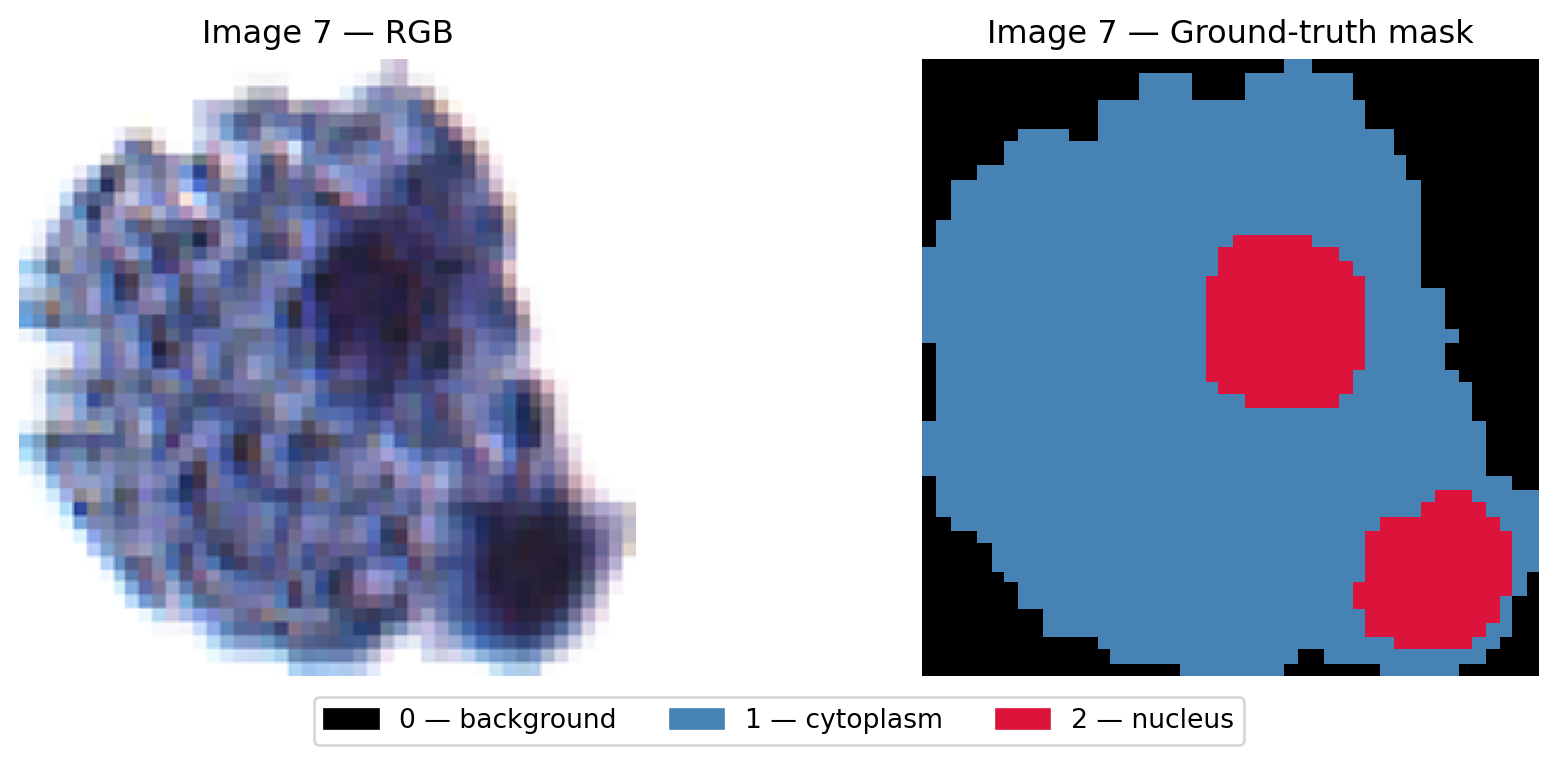
Before training anything, let’s check whether the three classes actually form separable clusters in RGB space. We use image 7 as a representative example — first viewing the raw image and its ground-truth mask, then projecting its pixels into colour space.
The key question: do background, cytoplasm, and nucleus pixels occupy different regions in colour space? If they do, a colour-based classifier has a chance.
Code
import jsonfrom IPython.display import HTML, displayIDX =7img7 = X[IDX] # (3, H, W) float32 0–1mask7 = y[IDX] # (H, W) 0/1/2pixels7 = img7.transpose(1, 2, 0).reshape(-1, 3) # (H*W, 3)labels7 = mask7.reshape(-1) # (H*W,)rng = np.random.default_rng(0)cls_colors = ['#333333', 'steelblue', 'crimson']cls_names = ['background', 'cytoplasm', 'nucleus']# ── Panel 1: raw image + ground-truth mask ────────────────────────────────────fig, axes = plt.subplots(1, 2, figsize=(10, 4))axes[0].imshow(img7.transpose(1, 2, 0))axes[0].set_title(f"Image {IDX} — RGB", fontsize=12)axes[0].axis('off')axes[1].imshow(mask7, cmap=mask_cmap, vmin=0, vmax=2, interpolation='nearest')axes[1].set_title(f"Image {IDX} — Ground-truth mask", fontsize=12)axes[1].axis('off')fig.legend(handles=legend_patches, loc='lower center', ncol=3, fontsize=10, bbox_to_anchor=(0.5, 0.0))plt.tight_layout(rect=[0, 0.07, 1, 1])plt.show()# ── Panel 2: 2-D colour-space projections ─────────────────────────────────────fig, axes = plt.subplots(1, 2, figsize=(12, 5))for cls inrange(3): samp = pixels7[labels7 == cls] n =min(3000, len(samp)) chosen = rng.choice(len(samp), n, replace=False) s = samp[chosen] axes[0].scatter(s[:, 0], s[:, 1], c=cls_colors[cls], s=1, alpha=0.5, label=cls_names[cls]) axes[1].scatter(s[:, 0], s[:, 2], c=cls_colors[cls], s=1, alpha=0.5, label=cls_names[cls])axes[0].set_xlabel('Red'); axes[0].set_ylabel('Green')axes[0].set_title('2-D projection — Red vs Green'); axes[0].legend(markerscale=6)axes[1].set_xlabel('Red'); axes[1].set_ylabel('Blue')axes[1].set_title('2-D projection — Red vs Blue'); axes[1].legend(markerscale=6)plt.tight_layout()plt.show()# ── Serialise for the 3-D widget below ───────────────────────────────────────pts = []for cls inrange(3): samp = pixels7[labels7 == cls] n =min(1500, len(samp)) sel = rng.choice(len(samp), n, replace=False) s = samp[sel] pts.append({'r': s[:, 0].round(4).tolist(),'g': s[:, 1].round(4).tolist(),'b': s[:, 2].round(4).tolist(),'color': cls_colors[cls],'name': cls_names[cls]})display(HTML(f'<script>window._ch5ColourData={json.dumps(pts)};</script>'))print(f"Image {IDX} — {pixels7.shape[0]:,} total pixels, "f"{sum(len(p['r']) for p in pts):,} sampled for 3-D colour space widget.")
Image 7 — 65,536 total pixels, 4,500 sampled for 3-D colour space widget.
The 2-D projections above each collapse one colour channel — you can only see two dimensions at a time. The interactive plot below shows all three channels simultaneously. Drag to rotate and find the angle where the three classes separate most cleanly.
NoteWhat to look for
If the three clouds of points are well-separated in 3-D, a k-NN classifier operating purely on colour should work well. Rotate the plot to find the viewing angle that best separates the classes. If the clouds overlap significantly, the classifier will make systematic errors at those boundary regions — and no amount of tuning k will fix the underlying ambiguity.
5.4 Flattening Training Images into a Pixel Matrix
To train k-NN we need every training pixel in a single table:
Feature matrixX_train_px: shape (total_pixels, 3) — each row is one pixel’s (R, G, B) values
Label vectory_train_px: shape (total_pixels,) — each entry is 0, 1, or 2
With a 256×256 image and ~130 training images, the full table would have ~8.5 million rows — training k-NN on all of them would be slow. We subsample — picking a fixed number of random pixels from each training image — to keep the problem manageable.
A naive uniform subsample mirrors each image’s natural class distribution, which is heavily skewed toward background (most of the image is empty space). To avoid training a classifier that barely ever sees nucleus pixels, we use stratified sampling: draw the same fixed quota from each class in every image.
Code
PIXELS_PER_CLASS =150# 150 pixels × 3 classes = 450 per training imagerng = np.random.default_rng(42)px_list = []lbl_list = []for i in train_idx: pixels = X[i].transpose(1, 2, 0).reshape(-1, 3) # (H*W, 3) lbls = y[i].reshape(-1) # (H*W,)for cls in [0, 1, 2]: cls_idx = np.where(lbls == cls)[0] # positions of this class n =min(PIXELS_PER_CLASS, len(cls_idx)) # guard: tiny regions chosen = rng.choice(cls_idx, n, replace=False) px_list.append(pixels[chosen]) lbl_list.append(lbls[chosen])X_train_px = np.vstack(px_list)y_train_px = np.hstack(lbl_list)print(f"Training pixel matrix : {X_train_px.shape} dtype: {X_train_px.dtype}")print(f"Training label vector : {y_train_px.shape}")# Class balance check — should be approximately equal across all three classesfor cls, name inenumerate(['background', 'cytoplasm', 'nucleus']): n = (y_train_px == cls).sum()print(f" {name:>12s}: {n:6d} ({100*n/len(y_train_px):.1f}%)")
Each image is 256×256 = 65,536 pixels. Background typically dominates — often 70–80% of the image is empty space around the cell. A uniform random sample of 500 pixels would therefore give the classifier ~375 background examples and only ~25 nucleus examples per image. Stratified sampling overrides this imbalance by enforcing equal quotas: 150 pixels per class per image. The classifier then sees the minority class (nucleus) as often as the majority class, which is especially important for getting accurate predictions in the clinically meaningful regions.
5.5 Method 1 — k-Nearest Neighbours
The k-NN classifier is the simplest of our four methods to describe and the most expensive to run. It is a lazy learner: training does nothing more than store the labelled pixels in memory. All of the work happens at prediction time. To classify a new query pixel, k-NN measures its Euclidean distance to every stored training pixel, picks the k closest, and returns whichever class label the majority of those k neighbours hold.
Quiz: The k-NN Method
Reading the description above, which of the following best describes the general method a k-Nearest Neighbours classifier uses to label a new query point?
5.5.1 Train the k-NN Classifier
KNeighborsClassifier stores the entire training set in memory. At prediction time, for each query pixel it:
Computes the Euclidean distance to every stored training pixel in 3-D colour space.
Identifies the n_neighbors closest stored pixels.
Returns the majority class label among those neighbours.
No learning happens during fit — the training data is the model. This is called a lazy learner.
NoteWhat “majority class label” means
After fit(), the model is just a lookup table of (R, G, B, label) tuples — the training pixels that were randomly sampled. The phrase “returns the majority class label among those neighbours” describes what happens at prediction time for each individual query pixel, not for the training pixels themselves.
For a single query pixel \(\mathbf{q} = (R, G, B)\), the classifier returns a single integer label \(\hat{y} \in \{0, 1, 2\}\):
where \(\mathcal{N}_k(\mathbf{q})\) is the set of \(k\) training pixels nearest to \(\mathbf{q}\) in Euclidean distance and \(y_i\) is the ground-truth label of training pixel \(i\).
When knn.predict() is called on all \(H \times W\) pixels of an image at once, it returns a flat array of \(H \times W\) integers — one label per pixel. Reshaping that array to \((H, W)\) gives the segmentation mask: a complete label map covering every pixel in the image, including pixels whose exact RGB colour was never seen during training.
Code
from sklearn.neighbors import KNeighborsClassifierknn = KNeighborsClassifier(n_neighbors=5, n_jobs=-1) # n_jobs=-1 → all CPU coresprint("Fitting k-NN classifier...")knn.fit(X_train_px, y_train_px)print("Done. The classifier has memorised all training pixels.")print(f"Number of stored training points: {len(X_train_px):,}")
Fitting k-NN classifier...
Done.  The classifier has memorised all training pixels.
Number of stored training points: 70,800
Quiz: k-NN Concept
When knn.predict() is called on a test image, what does the classifier do for each query pixel?
5.5.2 Choosing k
The number of neighbours \(k\) (set by n_neighbors) is the only hyperparameter in k-NN. It controls a fundamental trade-off between variance and bias:
\(k\)
Behaviour
Failure mode
Small (\(k = 1\))
Every query is decided by its single nearest training neighbour
High variance — a single mislabelled training pixel can corrupt all nearby predictions
Moderate (\(k = 5\)–\(15\))
Majority vote over a small neighbourhood smooths out isolated noise
Good balance for most problems
Large (\(k > 50\))
Vote taken from a very wide region of colour space
High bias — fine boundaries are blurred; large blobs of uniform colour replace crisp edges
This is the bias–variance trade-off: small \(k\) gives a wiggly, high-variance decision boundary that fits every quirk in the training data; large \(k\) gives a smooth, high-bias boundary that may miss genuine structure.
Choosing k via cross-validation
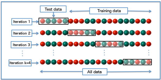
The principled approach is k-fold cross-validation on the training set. For each candidate \(k\), split the training pixels into \(F\) folds, train on \(F-1\) folds, and evaluate on the held-out fold. Average the Dice (or accuracy) score across folds, then pick the \(k\) that maximises it.
In k-fold cross-validation the data is split into \(k\) equal folds. Each iteration holds out one fold as the validation set and trains on the remaining \(k-1\) folds. Every data point is validated exactly once, giving a robust estimate of generalisation performance.
For each candidate \(k\):
from sklearn.model_selection import cross_val_scorefor k in [1, 3, 5, 7, 11, 15, 21]: clf = KNeighborsClassifier(n_neighbors=k, n_jobs=-1) scores = cross_val_score(clf, X_train_px, y_train_px, cv=5, scoring='accuracy')print(f"k={k:3d} accuracy = {scores.mean():.4f} ± {scores.std():.4f}")
A plot of validation accuracy vs \(k\) typically shows an elbow: rapid improvement from \(k = 1\) up to some moderate value, followed by a plateau or gentle decline. The elbow is the natural choice.
Rule of thumb:\(k \approx \sqrt{N_{\text{train}}}\) (where \(N_{\text{train}}\) is the number of training points) is a common starting point. With ~65,000 training pixels that gives \(k \approx 255\) — too large for boundary-heavy segmentation tasks. In practice, treat it as an upper bound and search from small values upward.
In this chapter we use n_neighbors = 5. Exercise 5.1 asks you to verify how the Dice score changes as \(k\) varies.
Quiz: Choosing k
A k-NN model trained with k = 1 achieves perfect accuracy on training data but Dice drops sharply on test images. Which explanation is correct?
5.5.3 Predicting Masks for Test Images
To predict a segmentation mask for a new image we:
Flatten the image from (H, W, 3) → (H*W, 3).
Pass all pixels at once to knn.predict().
Reshape the flat predictions back to (H, W).
How knn.predict() works
knn.predict() treats every pixel in the input image as a point in 3-D colour space and answers one question: given this (R, G, B) colour, what class do the nearest training pixels say it belongs to?
Step by step for one query pixel \(\mathbf{q} = (R, G, B)\):
Compute the Euclidean distance from \(\mathbf{q}\) to every stored training pixel \(\mathbf{x}_i\):
For an image with \(H \times W\) pixels, this procedure runs across all pixels in parallel (scikit-learn uses all CPU cores when n_jobs=-1), producing a flat array of \(H \times W\) class labels.
Non-sampled pixels (pixels from training images that were not selected during subsampling): the model has no record of them — it only stores the (R, G, B, label) pairs that were randomly drawn. When those pixels later appear as query points (e.g. if you run knn.predict() on a full training image to visualise the result), they are treated like any other input: the model finds their \(k\) nearest neighbours in the stored set and votes. A skipped pixel will be classified correctly as long as its colour falls near a well-represented region of colour space; it may be misclassified if it lies in a sparse or ambiguous region.
Test image pixels (pixels from images the model has never encountered): k-NN makes no distinction between a query from a training image and one from a test image. Every pixel is just a vector \((R, G, B)\). The model finds its nearest neighbours in the stored training set and votes. This is how k-NN generalises: it is not memorising spatial layouts or specific images — it is memorising a colour-to-class mapping. Any pixel whose colour falls in a region of colour space densely populated by, say, nucleus training pixels will be predicted as nucleus, regardless of which image it came from or where in that image it sits. The model’s generalisation ability therefore depends entirely on whether the training colour distribution is representative of the test colour distribution.
Try it: 2-D k-NN in action
The widget below lets you watch the k-NN vote happen for a single query pixel. We drop the blue channel and work in 2-D — so the decision is easy to see — using ~50 training points per class sampled from image 7. Drag the yellow query pixel across the plane (or use the R/G sliders), and change k with its slider. Training points that end up among the \(k\) nearest are highlighted with a ring, and thin lines trace the distances from the query to each neighbour. The shaded background shows the decision region for the current \(k\): the class the classifier would assign at every point on the plane.
Code
# ── Serialise 2-D (R, G) training data for the widget below ─────────────────_widget_rng = np.random.default_rng(0)widget_pts = []for cls inrange(3): samp = pixels7[labels7 == cls] n =min(50, len(samp)) sel = _widget_rng.choice(len(samp), n, replace=False) s = samp[sel, :2] # keep R, G only widget_pts.append({'r': s[:, 0].round(4).tolist(),'g': s[:, 1].round(4).tolist(),'class': cls,'color': cls_colors[cls],'name': cls_names[cls], })display(HTML(f'<script>window._ch5KnnWidget={json.dumps(widget_pts)};</script>'))print(f"Widget training data: {sum(len(p['r']) for p in widget_pts)} pixels from image {IDX} (R, G only).")
Widget training data: 150 pixels from image 7 (R, G only).
Quiz: 2-D k-NN in Action
In the 2-D k-NN widget above, you can change k with its slider. As you increase k from 1 to a much larger number while keeping the query pixel in the same place, what happens to the shaded decision regions — and why?
5.5.4 k-NN Test Performance
We now run k-NN on all test images and compute the mean Dice score across cytoplasm and nucleus — the two clinically meaningful classes. We will store these per-image scores so we can compare them against the other classifiers later.
Code
print("Running k-NN inference on all test images (may take a minute)...")knn_scores = []for i in test_idx: pred = predict_mask(X[i], knn) d = (dice_score(pred, y[i], 1) + dice_score(pred, y[i], 2)) /2 knn_scores.append(d)print(f"k-NN mean Dice (cyto+nuc): {np.mean(knn_scores):.4f} ± {np.std(knn_scores):.4f}")
Running k-NN inference on all test images (may take a minute)...
k-NN mean Dice (cyto+nuc): 0.7604  ±  0.1061
5.6 Method 2 — Logistic Regression
Where k-NN refuses to commit to any model — it just stores data and looks up neighbours — logistic regression does the opposite. It is a parametric, eager learner: at training time it fits a small set of weights, and at prediction time it does almost no work. The data is summarised by those weights and discarded.
For a two-class problem with input vector \(\mathbf{x} = (R, G, B)\), logistic regression models the probability of class 1 as:
\[P(y = 1 \mid \mathbf{x}) = \sigma(\mathbf{w} \cdot \mathbf{x} + b) = \frac{1}{1 + e^{-(w_R R + w_G G + w_B B + b)}}\]
The function \(\sigma\) is the logistic sigmoid, which squeezes any real number into \((0, 1)\) — the natural range for a probability. The decision boundary — the locus of points where the model is exactly 50 % confident — is the plane\(\mathbf{w} \cdot \mathbf{x} + b = 0\). Logistic regression therefore can only carve colour space into half-spaces with flat boundaries.
For three classes (background, cytoplasm, nucleus) we use the multi-class generalisation, softmax regression. The model fits one weight vector per class and the predicted probability of class \(c\) is:
The decision boundary between any pair of classes is again a plane in RGB space. Whatever non-linear structure the colour clouds may have, logistic regression can only fit it with planes — three planes in our case, meeting at a triple junction.
Code
from sklearn.linear_model import LogisticRegressionprint("Training Logistic Regression (softmax) on pixel RGB...")lr = LogisticRegression(max_iter=2000)lr.fit(X_train_px, y_train_px)print(f"Done. Coefficients shape: {lr.coef_.shape} (one row per class, one weight per channel)")print(f"Intercepts: {np.round(lr.intercept_, 3)}")# Per-image Dice on the test setprint("\nRunning Logistic Regression inference on all test images...")lr_scores = []for i in test_idx: pred = predict_mask(X[i], lr) d = (dice_score(pred, y[i], 1) + dice_score(pred, y[i], 2)) /2 lr_scores.append(d)print(f"LR mean Dice (cyto+nuc): {np.mean(lr_scores):.4f} ± {np.std(lr_scores):.4f}")
Training Logistic Regression (softmax) on pixel RGB...
Done. Coefficients shape: (3, 3)  (one row per class, one weight per channel)
Intercepts: [-31.42   14.067  17.353]

Running Logistic Regression inference on all test images...
LR mean Dice (cyto+nuc): 0.7788  ±  0.1229
NoteWhat the weights mean
Each row of lr.coef_ is a weight vector \(\mathbf{w}_c = (w_R, w_G, w_B)\) for one class. Positive weights say “more of this channel pushes the prediction toward this class”; negative weights say “more of this channel pushes the prediction away”. Combined with the intercepts, the three planes \(\mathbf{w}_c \cdot \mathbf{x} + b_c = \mathbf{w}_{c'} \cdot \mathbf{x} + b_{c'}\) partition RGB space into three regions. If the three colour clouds you saw earlier in the 3-D widget are even roughly linearly separable, LR will produce a Dice score close to k-NN’s — at a fraction of the prediction cost.
5.6.1 Try it: LR in 3-D Colour Space
For k-NN we used the 2-D widget above to watch the k nearest neighbours light up around a query pixel. For logistic regression there is nothing to look up — only the weights lr.coef_ and a final softmax. The widget below re-uses image 7’s RGB cloud as a backdrop and overlays the three pairwise decision planes the chapter’s lr actually fitted. Drag the R, G, B sliders to move a yellow query pixel through 3-D colour space.
Three things update together as you move:
The 3-D scatter shows which side of each plane the query lands on.
The softmax bars show \(p_c\) — the probability LR assigns to each class.
The sigmoid inset plots \(\sigma(z) = 1/(1 + e^{-z})\), with one coloured marker per class at \(z_c^{\mathrm{ovr}} = z_c - \mathrm{LSE}(z_{\bar c})\). The marker’s height equals \(p_c\) — visually demonstrating that softmax is just the multi-class sigmoid: a smooth squash from “linear evidence” onto \([0, 1]\).
Code
# ── Serialise LR weights and an image-7 RGB scatter for the widget below ────_lr_widget_rng = np.random.default_rng(7)_lr_pts = []for _cls inrange(3): _samp = pixels7[labels7 == _cls] _n =min(800, len(_samp)) _sel = _lr_widget_rng.choice(len(_samp), _n, replace=False) _s = _samp[_sel] _lr_pts.append({'r': _s[:, 0].round(4).tolist(),'g': _s[:, 1].round(4).tolist(),'b': _s[:, 2].round(4).tolist(),'color': cls_colors[_cls],'name': cls_names[_cls], })_lr_payload = {'coef': np.round(lr.coef_, 5).tolist(), # shape (3, 3)'intercept': np.round(lr.intercept_, 5).tolist(), # shape (3,)'class_colors': cls_colors,'class_names': cls_names,'scatter': _lr_pts,}display(HTML(f'<script>window._ch5LrModel={json.dumps(_lr_payload)};</script>'))print(f"LR widget data ready: {sum(len(p['r']) for p in _lr_pts)} pixels from image {IDX} + LR weights/intercepts.")
LR widget data ready: 2400 pixels from image 7 + LR weights/intercepts.
NoteWhat to try in the LR widget
Move the query into each of the three coloured clouds in turn — for example R = G = B ≈ 0.05 lands inside the nucleus cloud (one bar near 1.0, the matching sigmoid marker pinned at the top); R = G = B ≈ 0.85 lands in the background cloud; mid-grey R = G = B ≈ 0.45 lands in the cytoplasm cloud. Now slide the query into the boundary region between two clouds: two markers slide toward the centre of the sigmoid (around σ ≈ 0.5), and the predicted-class label snaps from one to the other the moment you cross a plane. The boundary is a single, flat plane in colour space — that flatness is exactly the limitation lr brings to this dataset.
Quiz: Logistic Regression
Why does logistic regression typically run much faster at prediction time than k-NN, even though it produced a similar mean Dice on this dataset?
5.7 Method 3 — Random Forest
A random forest is an ensemble of decision trees. Each tree is trained on a bootstrap sample of the training pixels (sampling with replacement), and at every internal node it picks a random subset of features and chooses the threshold on one of them that best splits the remaining pixels by class. The result is a forest of highly varied trees; predictions are made by majority vote across the forest.
A single decision tree partitions colour space into rectangular boxes by repeatedly asking “is \(R < 0.42\)?”, “is \(G > 0.31\)?”, and so on. Each tree’s decision regions are therefore axis-aligned and look like a Manhattan grid. A forest of such trees averages many of these grids — the resulting decision boundary is non-linear, can fit complex colour distributions, and is much smoother than any single tree’s. Random forests have three properties that make them attractive on this dataset:
Non-linear by default — they can carve colour space into curved-ish regions, unlike logistic regression’s planes.
Robust — bootstrapping and random feature selection make the forest resistant to a few mislabelled training pixels.
Fast at prediction time — once trained, each tree is a simple if/else cascade; no distance computation, no exponentials.
Code
from sklearn.ensemble import RandomForestClassifierprint("Training Random Forest (100 trees) on pixel RGB...")rf = RandomForestClassifier(n_estimators=100, random_state=42, n_jobs=-1)rf.fit(X_train_px, y_train_px)print(f"Done. Forest contains {len(rf.estimators_)} trees.")print(f"Mean tree depth: {np.mean([t.tree_.max_depth for t in rf.estimators_]):.1f}")print("\nRunning Random Forest inference on all test images...")rf_scores = []for i in test_idx: pred = predict_mask(X[i], rf) d = (dice_score(pred, y[i], 1) + dice_score(pred, y[i], 2)) /2 rf_scores.append(d)print(f"RF mean Dice (cyto+nuc): {np.mean(rf_scores):.4f} ± {np.std(rf_scores):.4f}")
Training Random Forest (100 trees) on pixel RGB...
Done. Forest contains 100 trees.
Mean tree depth: 32.4

Running Random Forest inference on all test images...
RF mean Dice (cyto+nuc): 0.7607  ±  0.1054
NoteFeature importances are a free by-product
Each tree in a random forest tracks which feature it splits on most often, and how much each split reduced impurity. Averaged across the forest, this gives feature importances — rf.feature_importances_ returns a 3-vector telling you which colour channel matters most for separating the classes on this dataset. With only three input features the importances are not very revealing, but in Chapter 7 we will use the same trick on a 30-dimensional hand-crafted feature vector and read off which texture and gradient features actually pull their weight.
5.7.1 Try it: Random Forest in 2-D Colour Space
Where logistic regression carves colour space with a small number of flat planes, a random forest carves it with many axis-aligned boxes. Each tree is built independently on its own bootstrap sample with random feature subsets, so the trees disagree about exactly where the boxes go. The forest’s prediction is the majority vote across the trees.
To make every step visible, we train a small forest of 50 trees on just the R and G channels of image 7’s pixels (a 2-D problem that is easy to draw). Drag the yellow query around the R-G plane — or use the R, G sliders — and watch three things move together:
The shaded background — the forest’s predicted class for every pixel of the plane. Slide Trees voting from 1 up to 50 and watch the boundary go from blocky and idiosyncratic (one tree’s whims) to smooth and stable (variance averaged out across many trees).
The thin grey lines — splits from one selected tree. Flip Show splits from tree # to compare different trees and notice that no two are alike.
The vote tally on the right — every voting tree’s vote on the query pixel, stacked by class. The class with the most votes wins.
Code
# ── Train a 2-D Random Forest on image 7's R/G features for the widget below ──from sklearn.ensemble import RandomForestClassifier as _RF2d_rf_widget_rng = np.random.default_rng(11)_rf_train_X, _rf_train_y, _rf_visible = [], [], []for _cls inrange(3): _samp = pixels7[labels7 == _cls][:, :2] # keep R, G only _n =min(220, len(_samp)) _sel = _rf_widget_rng.choice(len(_samp), _n, replace=False) _rf_train_X.append(_samp[_sel]) _rf_train_y.append(np.full(_n, _cls))# A smaller subset is drawn on the canvas to keep it readable _vis_n =min(70, _n) _vis_sel = _rf_widget_rng.choice(_n, _vis_n, replace=False) _rf_visible.append(_samp[_sel][_vis_sel])_rf_X = np.vstack(_rf_train_X)_rf_y = np.hstack(_rf_train_y)_rf2d = _RF2d(n_estimators=50, max_depth=6, random_state=42, n_jobs=-1)_rf2d.fit(_rf_X, _rf_y)def _serialize_tree(est): t = est.tree_ leaf_class = [int(np.argmax(v[0])) for v in t.value]return {'feature': t.feature.tolist(),'threshold': [float(round(x, 5)) for x in t.threshold.tolist()],'left': t.children_left.tolist(),'right': t.children_right.tolist(),'class': leaf_class, }_rf_payload = {'trees': [_serialize_tree(t) for t in _rf2d.estimators_],'class_colors': cls_colors,'class_names': cls_names,'visible_pts': [ {'r': float(round(x[0], 4)),'g': float(round(x[1], 4)),'cls': int(c)}for cls_idx, pts inenumerate(_rf_visible)for x, c inzip(pts.tolist(), [cls_idx] *len(pts)) ],}display(HTML(f'<script>window._ch5RfModel={json.dumps(_rf_payload)};</script>'))print(f"RF widget data ready: {len(_rf2d.estimators_)} trees on {len(_rf_X)} (R, G) pixels"f" from image {IDX}; {sum(len(p) for p in _rf_visible)} points drawn on the canvas.")
RF widget data ready: 50 trees on 660 (R, G) pixels from image 7; 210 points drawn on the canvas.
NoteWhat to try in the RF widget
Drop the Trees voting slider all the way down to 1: the shaded background becomes a single tree’s blocky decision map, often clearly different from the cluster centres. Now drag the slider up to 5, 10, 25, 50 — the boundary smooths in front of your eyes, because the trees that disagreed with the rough shape get out-voted by the trees that agreed. Park the query in a corner of the plane and flip Show splits from tree # through several values: every tree carves the plane differently because each one was trained on a different bootstrap sample with a random feature subset at each split. Finally, drag the query into the boundary between two clouds and watch the vote bar split: a 26 / 24 vote means the forest was nearly tied, which is exactly where errors will cluster on the test set.
Quiz: Random Forest
Compared with a single deep decision tree trained on the same pixels, what is the main reason a random forest of 100 trees gives a more reliable segmentation?
5.8 Method 4 — Multi-Layer Perceptron
A Multi-Layer Perceptron (MLP) is the simplest kind of neural network: a stack of fully-connected layers, each followed by a non-linear activation. With enough hidden units it can approximate any continuous decision surface in colour space — far more flexible than logistic regression’s planes or random forests’ axis-aligned boxes.
The architecture we will use here is intentionally tiny: 3 → 32 → 16 → 3. Three input units (R, G, B), two hidden layers with 32 and 16 ReLU units, and three output units that are passed through a softmax to produce class probabilities. The full forward pass for a single pixel is:
The weight matrices \(\mathbf{W}_1, \mathbf{W}_2, \mathbf{W}_3\) and biases are learned by gradient descent on a cross-entropy loss — the same machinery you will meet formally in Chapter 6. For now, scikit-learn’s MLPClassifier hides the optimisation and lets us treat the MLP as a drop-in classifier with the same fit / predict interface as the others.
Code
from sklearn.neural_network import MLPClassifierprint("Training MLP (3 → 32 → 16 → 3) on pixel RGB...")mlp = MLPClassifier( hidden_layer_sizes=(32, 16), activation='relu', solver='adam', max_iter=200, random_state=42,)mlp.fit(X_train_px, y_train_px)n_params =sum(W.size for W in mlp.coefs_) +sum(b.size for b in mlp.intercepts_)print(f"Done. Trainable parameters: {n_params}")print(f"Final training loss: {mlp.loss_:.4f} Iterations run: {mlp.n_iter_}")print("\nRunning MLP inference on all test images...")mlp_scores = []for i in test_idx: pred = predict_mask(X[i], mlp) d = (dice_score(pred, y[i], 1) + dice_score(pred, y[i], 2)) /2 mlp_scores.append(d)print(f"MLP mean Dice (cyto+nuc): {np.mean(mlp_scores):.4f} ± {np.std(mlp_scores):.4f}")
Training MLP (3 → 32 → 16 → 3) on pixel RGB...
Done. Trainable parameters: 707
Final training loss: 0.2852    Iterations run: 72

Running MLP inference on all test images...
MLP mean Dice (cyto+nuc): 0.7927  ±  0.1199
NoteA neural network is a stack of logistic regressions
You can read the MLP architecture above as three logistic regressions stacked end-to-end: each hidden layer is a linear transform followed by a non-linearity. Without the ReLU activations, the whole network would collapse algebraically into a single linear transform — equivalent to plain logistic regression. The non-linearities are what let the MLP bend its decision surfaces. We will explore this idea interactively in Chapter 6 using the TensorFlow Playground, where you can watch the boundary curve in real time as hidden layers are added.
Quiz: Multi-Layer Perceptron
The MLP above has roughly \(3 \times 32 + 32 \times 16 + 16 \times 3 \approx 700\) trainable weights, far more than logistic regression’s \(9\) weights. Yet on this dataset the MLP’s mean Dice is only marginally better than LR’s. Which explanation best fits this observation?
5.9 Comparing the Methods
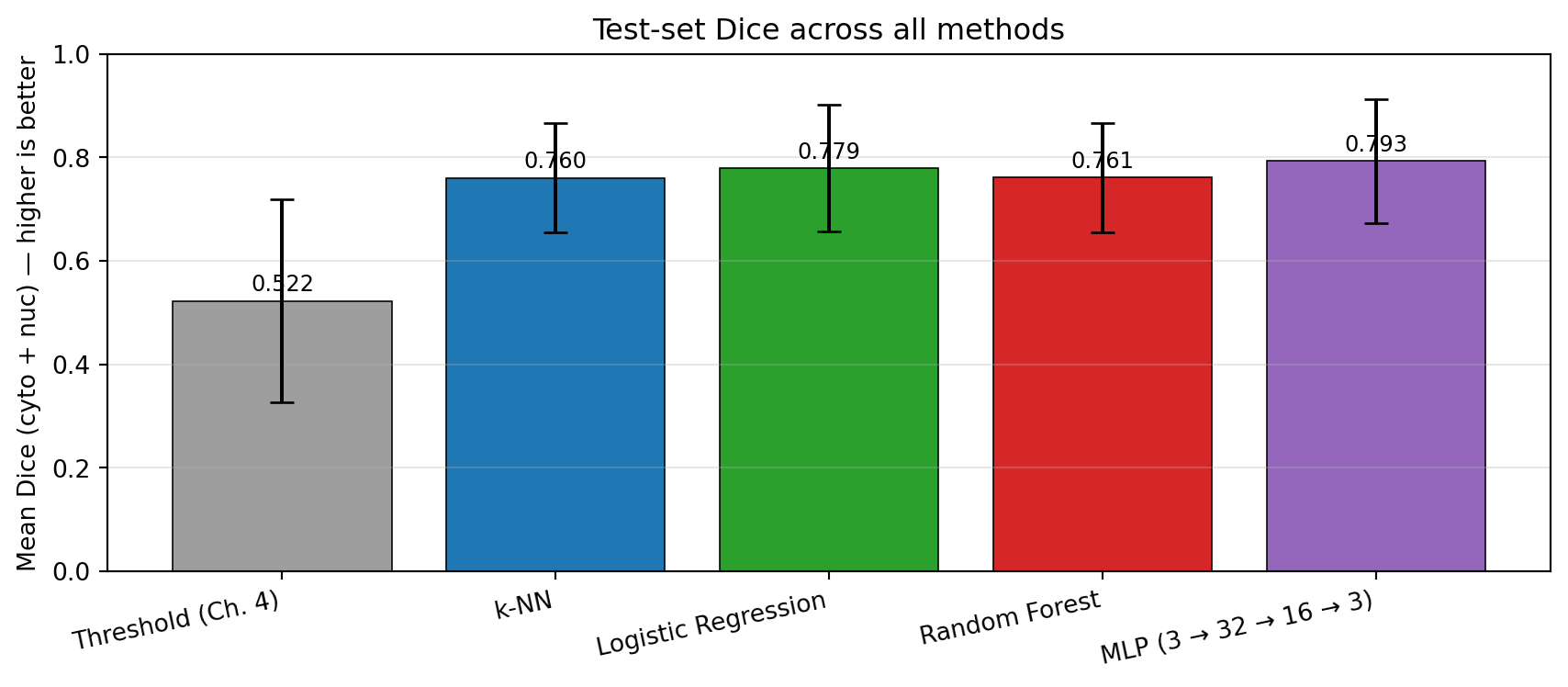
We now have five candidates for segmenting these images: the Chapter 4 grayscale threshold and the four ML classifiers from this chapter. To compare them on equal terms we run all five on the test set and report the mean Dice score across cytoplasm and nucleus.
Code
# Re-implement the Chapter 4 threshold rule for an apples-to-apples comparisondef segment_threshold(img, t_nucleus=0.3, t_cytoplasm_max=0.7): gray = img.mean(axis=0) # (3, H, W) → (H, W), values already in [0, 1] pred = np.zeros(gray.shape, dtype=np.int64) pred[gray < t_nucleus] =2 pred[(gray >= t_nucleus) & (gray <= t_cytoplasm_max)] =1return predthresh_scores = []for i in test_idx: pred = segment_threshold(X[i]) d = (dice_score(pred, y[i], 1) + dice_score(pred, y[i], 2)) /2 thresh_scores.append(d)results = {'Threshold (Ch. 4)': thresh_scores,'k-NN': knn_scores,'Logistic Regression': lr_scores,'Random Forest': rf_scores,'MLP (3 → 32 → 16 → 3)': mlp_scores,}print(f"{'Method':<28}{'Mean Dice':>10}{'Std':>8}")print('='*55)for name, scores in results.items():print(f"{name:<28}{np.mean(scores):>10.4f}{np.std(scores):>8.4f}")print('='*55)
The numbers tell a clear story: all four ML methods improve over thresholding, and they cluster together within a narrow band. The differences among the four learners are smaller than the spread within any single method’s per-image scores. The ranking can shift between runs, but the structure does not — the gap between threshold and any ML method is much larger than the gap between the ML methods themselves.
Code
fig, ax = plt.subplots(figsize=(9, 4))methods =list(results.keys())means = [np.mean(s) for s in results.values()]stds = [np.std(s) for s in results.values()]colors = ['#9e9e9e', '#1f77b4', '#2ca02c', '#d62728', '#9467bd']bars = ax.bar(methods, means, yerr=stds, color=colors, capsize=5, edgecolor='black', linewidth=0.6)ax.set_ylabel('Mean Dice (cyto + nuc) — higher is better')ax.set_ylim(0, 1)ax.set_title('Test-set Dice across all methods', fontsize=12)for bar, m inzip(bars, means): ax.text(bar.get_x() + bar.get_width() /2, bar.get_height() +0.02,f'{m:.3f}', ha='center', fontsize=9)ax.grid(axis='y', alpha=0.3)plt.xticks(rotation=12, ha='right')plt.tight_layout()plt.show()
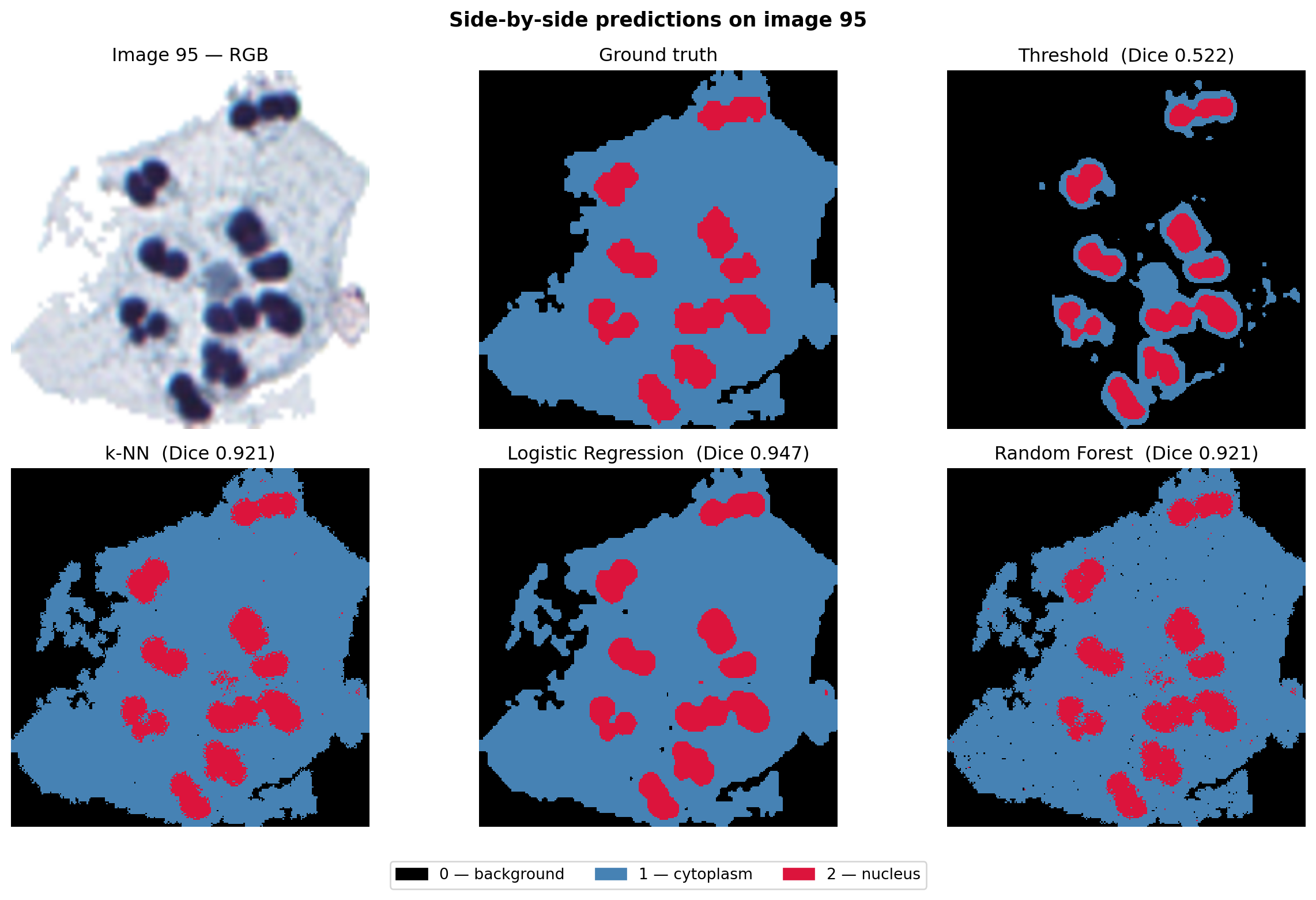
To see where the methods agree and disagree, we visualise the predicted masks side-by-side for one representative test image:
Notice that the four ML masks look qualitatively similar to one another — and qualitatively different from the threshold mask. The threshold mask hugs intensity contours; the ML masks all pick out the nucleus and cytoplasm in roughly the same places, with similar speckle artefacts. They share strengths and weaknesses, because they all look at the same input.
Quiz: Why the Methods Cluster
Looking at the bar chart and the side-by-side prediction maps, why do the four very different ML algorithms (k-NN, LR, RF, MLP) end up with such similar Dice scores and visually similar masks?
5.10 Why All Colour-Only Methods Hit a Ceiling
The Chapter 4 threshold was a hard rule on a single luminance value. The four classifiers in this chapter are progressively more flexible: a memorised lookup table (k-NN), a fitted plane (LR), an ensemble of axis-aligned splits (RF), and a non-linear neural network (MLP). Yet their Dice scores cluster within a few percentage points of each other, and the side-by-side masks share the same qualitative defects. Why?
They all see the same input. Each classifier consumes a single pixel’s three RGB values and outputs a class label. None of them looks at the pixel’s row, column, or neighbours. A nucleus pixel at the boundary of the nucleus has the same RGB colour as one buried at the centre, and a stray bright pixel in the cytoplasm has the same colour as a true background pixel. The information needed to disambiguate these cases is not in the feature vector — so no choice of classifier can recover it.
This produces two characteristic, shared failure modes:
Speckle noise — isolated wrong-class pixels scattered throughout otherwise-correct regions, because the classifier has no smoothing from spatial neighbours.
Boundary errors — at the edges of the nucleus and cytoplasm, where colours blend continuously across the boundary, the classifier has to commit to one class on colour alone. The result is a noisy, ragged contour rather than a smooth edge.
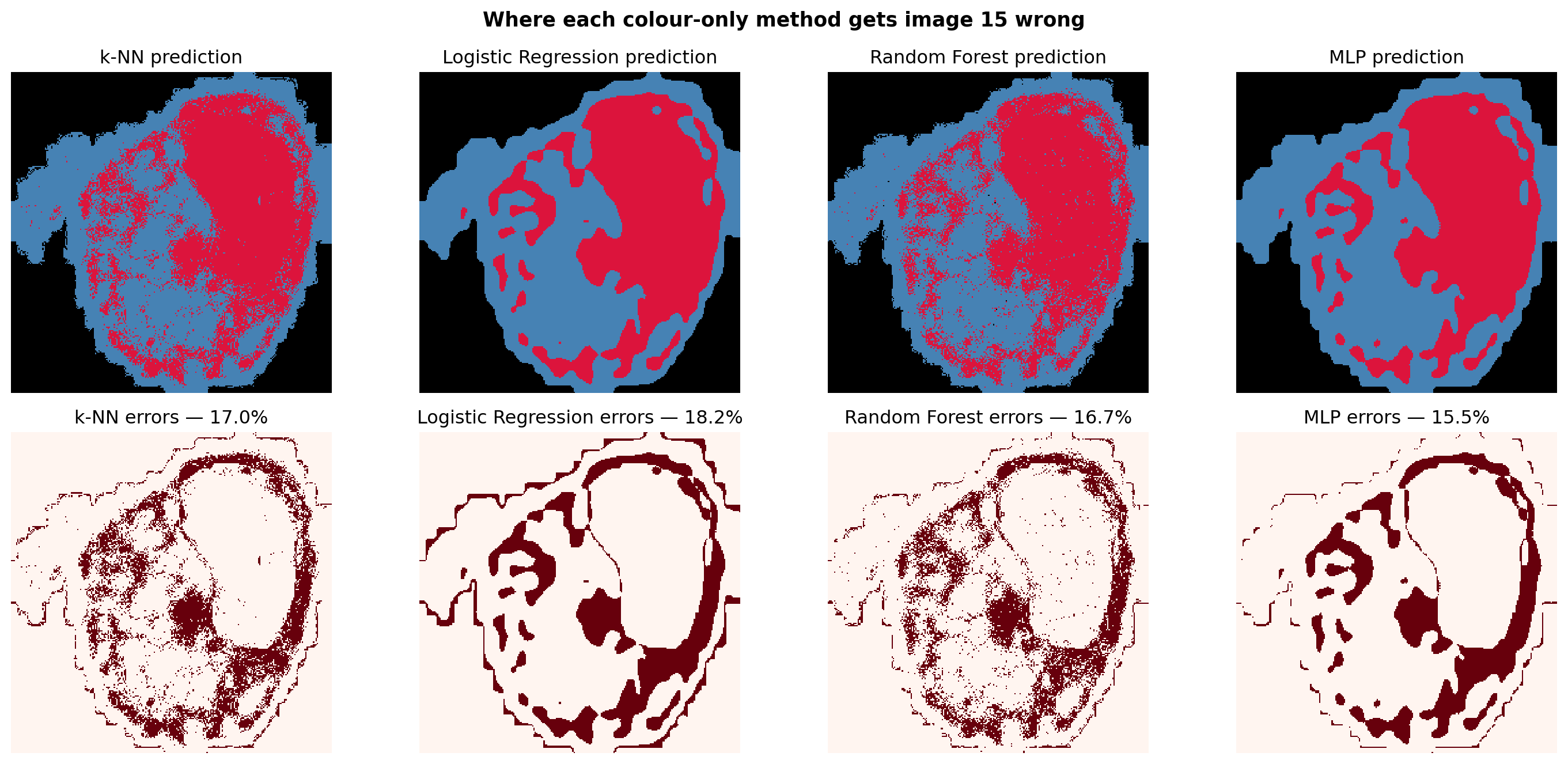
The error maps below visualise this for one test image, comparing all four ML methods on the same image.
Code
idx = test_idx[1]fig, axes = plt.subplots(2, 4, figsize=(15, 7))preds = {'k-NN': predict_mask(X[idx], knn),'Logistic Regression': predict_mask(X[idx], lr),'Random Forest': predict_mask(X[idx], rf),'MLP': predict_mask(X[idx], mlp),}for col, (name, pred) inenumerate(preds.items()): err = (pred != y[idx]) axes[0, col].imshow(pred, cmap=mask_cmap, vmin=0, vmax=2, interpolation='nearest') axes[0, col].set_title(f"{name} prediction"); axes[0, col].axis('off') axes[1, col].imshow(err, cmap='Reds', interpolation='nearest') axes[1, col].set_title(f"{name} errors — {err.mean()*100:.1f}%") axes[1, col].axis('off')plt.suptitle(f"Where each colour-only method gets image {idx} wrong", fontsize=13, fontweight='bold')plt.tight_layout()plt.show()print("Notice how the red error pixels for all four methods cluster in the SAME places —")print("at the cell boundary and inside textured cytoplasm regions. Different classifiers,")print("same blind spot: no spatial context, no way out.")
Notice how the red error pixels for all four methods cluster in the SAME places —
at the cell boundary and inside textured cytoplasm regions. Different classifiers,
same blind spot: no spatial context, no way out.
NoteSpatial context: the missing ingredient
Every classifier in this chapter treats each pixel as an independent 3-vector. A nucleus pixel at the very edge of the nucleus has the same RGB colour as one near the centre — but they sit in very different neighbourhoods. To break through the ceiling we need features that describe what surrounds a pixel, not just the pixel itself.
Two complementary moves fix this, and they form the next three chapters of the book:
Chapter 6 introduces neural networks formally — how a network with hidden layers, gradient descent, and backpropagation can learn arbitrarily flexible decision boundaries. That gives us the tool but not yet the input it needs to win.
Chapter 7 keeps the classifiers from this chapter but feeds them richer features — gradient magnitudes, Gabor filter responses, GLCM texture statistics — that summarise a pixel’s local neighbourhood. The same logistic regression and random forest, given those features, climb well past the ceiling we just hit.
Chapter 8 combines both ideas. Convolutional neural networks learn neighbourhood features and a flexible classifier together, end-to-end, from labels alone — and they finally close the gap to expert human segmentation.
Quiz: The Common Ceiling
All four classifiers in this chapter — k-NN, Logistic Regression, Random Forest, and MLP — produce visually similar errors and Dice scores within a few points of each other. Which statement best identifies the underlying limitation they share?
5.11 Summary
Method
Type
Decision boundary in RGB
Train
Predict
Threshold (Ch. 4)
hard rule
one luminance cut
none
trivial
k-NN
non-parametric, lazy
piecewise — Voronoi cells
trivial (just stores data)
slow (distance to all stored pixels)
Logistic Regression
parametric, linear
three planes meeting at a junction
fast (~9 weights)
very fast (one dot product)
Random Forest
non-parametric, ensemble
~axis-aligned, many curved-ish steps
medium (100 trees)
fast (tree traversal)
MLP (3 → 32 → 16 → 3)
parametric, non-linear
smooth curved surfaces
medium (gradient descent)
fast (matrix multiplies)
Key takeaways:
Treating segmentation as pixel classification unlocks the full RGB feature vector and gives every method substantially better Dice than the Chapter 4 grayscale threshold.
Among the four ML methods, flexibility alone does not buy much. k-NN, LR, RF, and MLP cluster within a narrow band — the gap between them is smaller than the gap between any of them and thresholding.
The common ceiling is the input, not the classifier. All four methods see only the three RGB values of a single pixel; none of them knows where the pixel sits or what surrounds it.
The path forward is twofold: better classifiers (Chapter 6 introduces neural networks formally; Chapter 8 builds CNNs) and better features (Chapter 7 hand-crafts spatial features; Chapter 8 lets the network learn them).
5.12 Exercises
Exercise 5.1 — Varying k in k-NN
The number of neighbours k is the only hyperparameter of k-NN. Too small (k = 1) → noisy; too large → over-smoothed boundaries.
Test k ∈ {1, 10, 25}. For each value, retrain the classifier and compute the mean Dice on the first 5 test images. Plot the error map for one image.
Which value of k gives the best Dice?
Does the error map look more or less speckly as k increases? Why?
Exercise 5.2 — Decision boundaries on the 3-D widget
Train each of the four classifiers (k-NN, LR, RF, MLP) on the same (R, G) 2-D pixels used in the k-NN widget, then sweep a fine (R, G) grid through predict() for each model. Plot the four resulting decision maps side by side.
Which classifier produces the smoothest boundaries? Which produces the most jagged?
Is there a region of (R, G) space where two classifiers disagree by more than 50 % of the pixels? What does that disagreement tell you about the colour clouds?
Exercise 5.3 — Adding spatial features
Modify the pixel feature vector to include the pixel’s (row, col) position alongside its RGB values, giving a 5-D feature vector. Retrain all four classifiers and compare the new mean Dice against the baseline.
Which classifier gains the most from adding spatial coordinates? Why might that be?
Do the segmentations look more spatially coherent? What is the downside of including raw position?
Exercise 5.4 — MLP architecture
The MLP in this chapter has hidden layers (32, 16). Try (8,), (64, 32), and (128, 64, 32). For each, report:
Training loss and number of iterations.
Mean Dice on the test set.
Whether the extra capacity actually helps. If it does not, what does that suggest about the limit imposed by the input features?
Exercise 5.5 — Random Forest feature importance
Train a Random Forest on (R, G, B) and inspect rf.feature_importances_. Repeat after augmenting the feature vector with the per-pixel grayscale value ((R + G + B) / 3) and the per-pixel red-blue ratio (R / (B + 1e-3)). Which engineered features earn high importance scores? Does adding them improve Dice, or does the forest already extract that information from the raw channels?
Exercise 5.6 — Class balance check
Inspect the class balance in y_train_px. If one class dominates, the classifier may be biased toward it. Try passing class_weight='balanced' to Logistic Regression and Random Forest and rerun the test-set evaluation. Does the rebalanced classifier help cytoplasm Dice without hurting nucleus Dice? Which classifier benefits most? KNeighborsClassifier does not accept class_weight — look at the scikit-learn docs and suggest an alternative strategy that achieves the same effect.