6 Introduction to Neural Networks
6.1 Overview
Neural networks have revolutionized machine learning and artificial intelligence over the past decade. Inspired by biological neurons in the brain, artificial neural networks are mathematical models composed of interconnected nodes (neurons) organized in layers. A signal flows from input to output through weighted connections, and these weights are adjusted during training to minimize prediction errors.
6.2 Historical Context and Modern Applications
The field of neural networks has a rich history spanning over 70 years. Early work by McCulloch and Pitts in the 1940s established the mathematical foundations. The perceptron algorithm of the 1960s showed that simple networks could learn. However, research stagnated in the 1970s and 1980s due to limitations in computing power and understanding. The “deep learning revolution” began around 2011 when Geoffrey Hinton’s team won a major image recognition competition using deep convolutional neural networks trained on GPUs.
Today, neural networks power some of the most transformative AI applications:
Computer Vision: Convolutional Neural Networks (CNNs) recognize objects in images, enabling facial recognition, medical imaging diagnosis, autonomous vehicles, and facial unlocking on phones.
Natural Language Processing: Transformer-based models like GPT (Generative Pre-trained Transformer) have revolutionized language understanding and generation. Modern Large Language Models (LLMs) like ChatGPT, Claude, and Gemini can engage in nuanced conversations, translate languages, summarize documents, write code, and answer questions across almost any domain. These models are trained on billions of parameters and can perform complex reasoning tasks.
Speech Recognition: Recurrent Neural Networks (RNNs) and their variants process sequential audio data, enabling voice assistants like Siri and Alexa.
Game Playing: Deep reinforcement learning networks have defeated world champions in chess, Go, and other strategic games by learning to predict and evaluate future game states.
Recommendation Systems: Neural networks power Netflix recommendations, YouTube suggestions, and social media feeds by learning patterns in user behavior and content.
Generative AI: Beyond text, neural networks generate images (DALL-E, Midjourney), music, and video, creating entirely new content from learned patterns.
6.3 The Diversity of Neural Network Architectures
Different problem types require different network architectures:
Feedforward Neural Networks are the basic architecture where information flows strictly from input to output through hidden layers. They excel at classification and regression tasks with fixed-size inputs.
Convolutional Neural Networks (CNNs) are specialized for image and spatial data. They use convolutional layers with learnable filters that detect local patterns (edges, textures, shapes) at multiple scales. The hierarchical structure—detecting edges first, then shapes, then objects—mirrors how humans perceive images.
Recurrent Neural Networks (RNNs) are designed for sequential data like time series, text, and speech. They maintain internal state (memory) that updates as they process each element in a sequence. This allows them to capture dependencies across time. Variants like LSTM (Long Short-Term Memory) and GRU (Gated Recurrent Unit) address the challenge of learning long-range dependencies.
Transformers are the modern breakthrough for sequence processing, especially language. Rather than processing data sequentially, transformers use “attention mechanisms” that allow the network to focus on relevant parts of the input. This enables parallel processing and handling of very long sequences. Transformers power most modern LLMs.
Autoencoders learn compressed representations of data by encoding inputs to a bottleneck layer, then reconstructing them from this compressed representation. They’re useful for dimensionality reduction and anomaly detection.
Generative Adversarial Networks (GANs) pit two networks against each other: a generator that creates fake data and a discriminator that judges authenticity. This competition drives both to improve, enabling realistic image and data generation.
6.4 Why Study Fundamentals?
With such powerful applications available, why study neural networks from scratch? Because understanding the fundamentals is crucial for:
- Designing effective architectures for your specific problem
- Debugging why models fail instead of blindly tuning hyperparameters
- Knowing when simpler models suffice instead of over-engineering
- Understanding trade-offs between model capacity, data requirements, and computational cost
- Implementing novel ideas and staying on the frontier of AI research
In this chapter, we’ll build understanding from the ground up using interactive exploration in the TensorFlow Playground. You’ll start with simple datasets and gradually discover why neural networks are necessary, how they work, and what makes them tick.
7 Anatomy of a Neural Network
7.1 The Basic Structure
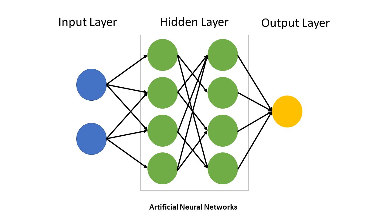
A neural network consists of layers of interconnected nodes (neurons). Let’s build understanding from the ground up.
7.1.1 Layers
A neural network typically has three types of layers:
Input Layer: The entry point for data - Contains one node per input feature - For a 2D classification problem: 2 input nodes (x₁ and x₂) - No computation happens here; it’s just the raw data
Hidden Layers: Intermediate processing layers (optional) - Between input and output - Perform nonlinear transformations of the input data - Can have any number of hidden layers and nodes per layer - Each node combines inputs through weighted sum and applies activation function
Output Layer: The final prediction - For binary classification: 1 output node - For multi-class classification: multiple output nodes (one per class) - Applies activation function appropriate to the task
7.1.2 Nodes and Connections
Each node in a hidden or output layer: - Receives input from all nodes in the previous layer - Multiplies each input by a weight - Sums the weighted inputs plus a bias term - Applies an activation function - Sends output to all nodes in the next layer
7.1.3 The Computation at Each Node
At a node in a hidden layer, the calculation is:
\[z = \sum_{i=1}^{n} w_i x_i + b\]
where: - \(x_i\) are the inputs to this node - \(w_i\) are the weights (parameters we’ll learn) - \(b\) is the bias (another learnable parameter) - \(z\) is the pre-activation value
Then we apply an activation function:
\[a = \sigma(z) = \sigma\left(\sum_{i=1}^{n} w_i x_i + b\right)\]
where \(\sigma\) is the activation function (we’ll explore several).
7.1.4 Example: A Simple Network
Consider a network for 2D classification: - Input layer: 2 nodes (x₁, x₂) - Hidden layer: 3 nodes - Output layer: 1 node
At the first hidden node: \[z_1 = w_{11} x_1 + w_{12} x_2 + b_1\] \[a_1 = \sigma(z_1)\]
At the output node (which might use sigmoid for binary classification): \[z_{out} = w_{out,1} a_1 + w_{out,2} a_2 + w_{out,3} a_3 + b_{out}\] \[\hat{y} = \sigma(z_{out})\]
This is how information flows: forward pass or forward propagation.
8 Training Neural Networks
8.0.1 The Loss Function
To train a network, we need to measure how wrong it is. The loss function quantifies the error between our prediction \(\hat{y}\) and the true label \(y\).
For binary classification, we use Binary Cross-Entropy:
\[L = -\left[y \log(\hat{y}) + (1-y) \log(1-\hat{y})\right]\]
For a batch of samples, we average over all samples:
\[E = \frac{1}{m} \sum_{i=1}^{m} L_i\]
where \(m\) is the number of samples in the batch.
The goal of training is to find weights and biases that minimize this loss.
8.0.2 Backpropagation: Computing Gradients
Once we know the loss, we need to update the weights to reduce it. The question is: in which direction should we move?
Backpropagation is the algorithm that computes the gradient of the loss with respect to each weight. It uses the chain rule from calculus, working backwards from the output to the input.
The key insight: - Loss depends on output → output depends on hidden layer → hidden layer depends on weights - By chaining these dependencies, we can compute how much each weight contributed to the loss - This tells us the direction to adjust each weight
We won’t derive the full algorithm here, but the result is: for each weight \(w\), we compute \(\frac{\partial L}{\partial w}\), which tells us the gradient (rate of change of loss with respect to that weight).
8.0.3 Gradient Descent: Updating Weights
Once we have the gradient, we update weights in the opposite direction:
\[w_{new} = w_{old} - \alpha \frac{\partial L}{\partial w}\]
where \(\alpha\) is the learning rate (how big a step to take).
We repeat this process: 1. Forward pass: compute predictions 2. Compute loss 3. Backpropagation: compute gradients 4. Update weights using gradient descent 5. Repeat until convergence
8.0.4 Epochs and Batch Size
In practice, we don’t update weights on just one sample. Instead:
- Batch: a subset of the training data (e.g., 32 samples)
- Epoch: one complete pass through all training data
If we have 1000 training samples and batch size 32: - One epoch = 1000/32 ≈ 31 batches - In one epoch, we do 31 weight updates - After one epoch, all 1000 samples have been used once
Mini-batch gradient descent: We typically use batches because: - More efficient computation (using matrix operations) - Smoother gradient estimates (average over multiple samples) - Better generalization (noise from mini-batches acts as regularization)
9 Linear Classification with the Gaussian Dataset
9.1 Introduction to the Gaussian Dataset
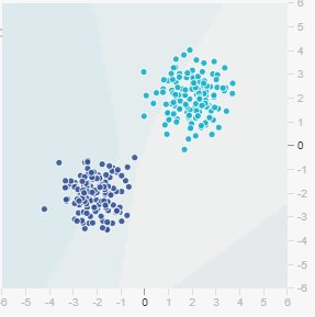
The TensorFlow Playground provides synthetic datasets for exploring neural networks. Let’s start with the simplest: the Gaussian dataset.
This dataset consists of two classes: - Class 0 (dark blue): scattered points in the first quadrant - Class 1 (light blue): scattered points in the third quadrant
Key observation: The classes are linearly separable. A straight line can perfectly separate them.
9.2 Understanding the Question Framework
For the next set of questions: 1. Open https://playground.tensorflow.org 2. Select Data: Gaussian 3. Follow the setup instructions for each question 4. Train the network and observe convergence 5. Answer the question based on your observations 6. Read the detailed feedback
Convergence criterion: We’ll consider convergence achieved when test loss drops below 0.02.
9.5 Question 1B: Adding More Features
Setup
Hidden Layers: None (0 layers)
Features: X₁, X₂, X₁², X₂² (select all)
Learning Rate: 0.001
Other settings: Same as Q1A
Train the network and compare: How many epochs until test loss ≤ 0.02 now?
Since X₁ alone perfectly separates the Gaussian clusters, what happens when you add all available features (X₁, X₂, X₁², X₂²)?
9.6 Question 1C: Comparing Network Depths
Setup
Features: X₁ only
Learning Rate: 0.001
Activation: ReLU
Other settings: Same as Q1A
Train three networks:
1. No hidden layers (linear): Note epochs to convergence
2. One hidden layer (4 neurons): Note epochs to convergence
3. Two hidden layers (4 neurons each): Note epochs to convergence
When you add hidden layers to the Gaussian classifier, what do you observe?
10 Nonlinear Problems and Activation Functions
10.1 When Linear Models Fail
So far, we’ve explored linearly separable problems where a simple linear classifier works perfectly. But what happens when classes are not linearly separable?
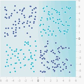
Consider this scenario: you want to classify points based on whether both features have the same sign (both positive or both negative) or opposite signs. This is the Exclusive OR (XOR) problem:
- Class 0 (dark blue): Both coordinates have the same sign
- Quadrant 1: x₁ > 0, x₂ > 0 ✓
- Quadrant 3: x₁ < 0, x₂ < 0 ✓
- Class 1 (light blue): Coordinates have opposite signs
- Quadrant 2: x₁ < 0, x₂ > 0 ✗
- Quadrant 4: x₁ > 0, x₂ < 0 ✗
No single straight line can separate these classes! You would need at least two lines, forming an “X” or “bowtie” pattern.
10.2 The Role of Activation Functions
This is where activation functions become essential.
Recall the computation at a hidden layer node:
\[z = w_1 x_1 + w_2 x_2 + b\]
Without an activation function, the output is simply \(z\) (linear). If you stack multiple linear layers:
\[\text{Layer 2} = W_2 (\text{Layer 1}) = W_2 (W_1 x) = (W_2 W_1) x\]
This is just matrix multiplication—still linear! You need an activation function to introduce nonlinearity.
An activation function \(\sigma(z)\) applies a nonlinear transformation:
\[\text{Hidden output} = \sigma(w_1 x_1 + w_2 x_2 + b)\]
Now each hidden layer can learn nonlinear features of the input. Multiple hidden layers can learn increasingly abstract representations.
10.3 Exploring the XOR Problem
The XOR problem cannot be solved by: - A linear classifier (single straight line) - Any number of linear layers (still equivalent to one linear transformation)
But it CAN be solved by: - A hidden layer with nonlinear activation function - Feature engineering (creating features like \(x_1 x_2\))
12 Activation Functions Compared
12.1 Question 3: Comparing ReLU, Sigmoid, and Tanh
Setup Part 1: ReLU
Hidden Layers: 1 layer with 4 neurons
Features: X₁, X₂ only
Learning Rate: 0.001
Activation: ReLU
Train and record: Epochs until test loss ≤ 0.02
Setup Part 2: Sigmoid
Change Activation to Sigmoid, keep everything else the same
Train and record: Epochs until test loss ≤ 0.02
Setup Part 3: Tanh
Change Activation to Tanh, keep everything else the same
Train and record: Epochs until test loss ≤ 0.02
Based on your experiments with ReLU, Sigmoid, and Tanh, which statement best describes activation function performance on XOR?
12.2 Understanding the Activation Functions
12.2.1 ReLU (Rectified Linear Unit)
\[\text{ReLU}(z) = \max(0, z) = \begin{cases} z & \text{if } z > 0 \\ 0 & \text{if } z \leq 0 \end{cases}\]
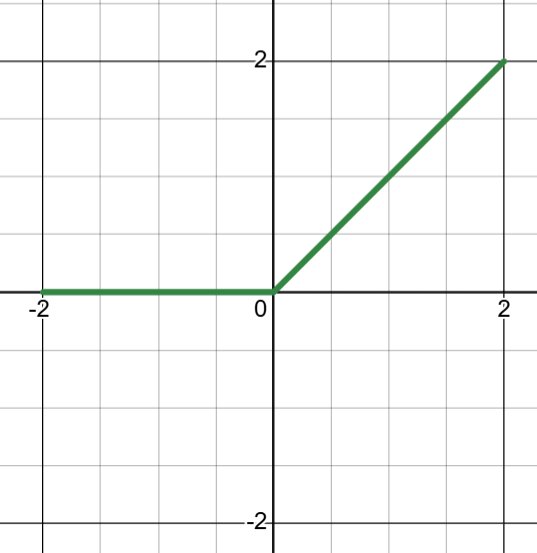
Derivative: 1 when \(z > 0\), 0 otherwise
Advantages: - Computationally simple - Preserves gradient magnitude (derivative is 0 or 1) - Avoids vanishing gradient problem - Leads to sparse activations (many neurons output 0)
Disadvantages: - “Dead ReLU” problem: neurons with \(z < 0\) always output 0 and their gradients are 0
12.2.2 Sigmoid
\[\sigma(z) = \frac{1}{1 + e^{-z}}\]
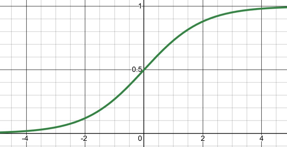
Derivative: \(\sigma(z)(1 - \sigma(z))\) with maximum of 0.25
Advantages: - Smooth, differentiable everywhere - Output range (0, 1) is intuitive for probabilities - Good for binary classification output layer
Disadvantages: - Vanishing gradient problem: derivatives near 0 when \(|z|\) is large - Not zero-centered: outputs are always positive - Slower training in deep networks
12.2.3 Tanh (Hyperbolic Tangent)
\[\tanh(z) = \frac{e^z - e^{-z}}{e^z + e^{-z}}\]
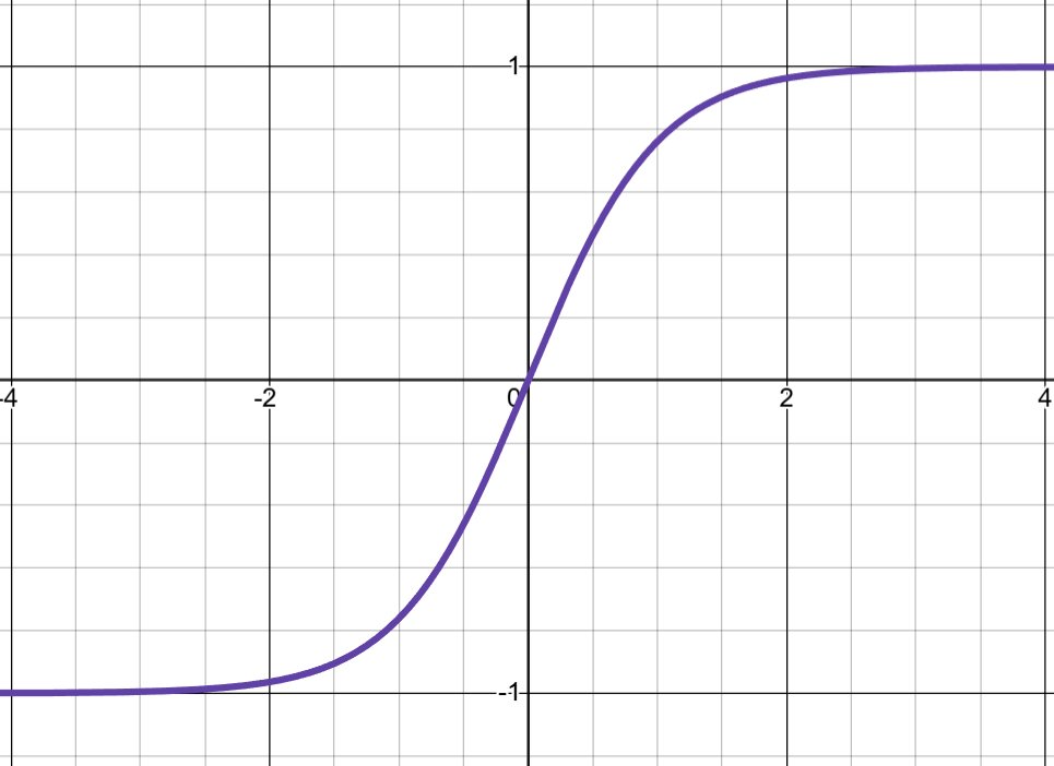
Derivative: \(1 - \tanh^2(z)\) with maximum of 1
Advantages: - Similar to Sigmoid but zero-centered (output range -1 to 1) - Smoother than ReLU, can be better for small networks - Larger derivatives than Sigmoid (less severe vanishing gradients)
Disadvantages: - Still suffers from vanishing gradients (though less than Sigmoid) - Slower than ReLU on most problems - More complex computation than ReLU
13 The Role of Initialization and Randomness
13.1 Why Neural Networks Don’t Always Converge the Same Way
So far, we’ve treated neural network training as deterministic: give it a dataset and a learning rate, and it will converge. But in reality, training has a crucial stochastic (random) component that can dramatically affect the outcome.
13.2 The Role of Weight Initialization
When a neural network begins training, its weights and biases start with random values. This initialization is crucial for several reasons:
Breaking Symmetry: If all neurons in a hidden layer started with identical weights, they would learn identical features during training. Randomization ensures each neuron develops different, specialized features.
Escaping Bad Local Minima: The loss surface is not convex. It contains many local minima—places where the gradient is zero but the loss is not globally optimal. Good random initialization helps the network start in regions that lead to better solutions.
Setting the Scale: The magnitude of initial weights affects how quickly the network learns. Too large and gradients explode; too small and learning stalls. Proper initialization schemes (like Xavier or He initialization) carefully choose weight magnitudes based on the number of inputs and outputs.
Stochasticity in Mini-Batches: Each epoch, the training data is randomly shuffled and divided into mini-batches. Different orderings can lead to different learning trajectories, causing small variations in final performance.
Random Dropout and Noise: Modern techniques deliberately add randomness (dropout, noise injection) to prevent overfitting and improve generalization.
13.3 Question 4: Does Convergence Always Look the Same?
Setup
Hidden Layers: 1 layer with 3 neurons
Features: X₁, X₂ only
Learning Rate: 0.01
Activation: ReLU
Batch Size: Default
Regularization: None
Noise: 0
Important: Click the reload button (circular arrow icon) several times.
Each reload reinitializes the weights randomly and reshuffles the batches.
Observe: Do you get the same convergence curve every time?
When you click reload multiple times on the XOR problem with fixed hyperparameters, what do you observe?
13.4 Understanding Initialization
Weight initialization strategies determine how the random starting values are chosen:
Random Normal: Weights drawn from a normal distribution. Simple but can cause vanishing or exploding gradients.
Xavier/Glorot Initialization: Scale weights based on number of inputs: \(w \sim \text{Uniform}\left(-\sqrt{\frac{6}{n_{in} + n_{out}}}, \sqrt{\frac{6}{n_{in} + n_{out}}}\right)\). This balances signal propagation through the network.
He Initialization: For ReLU networks: \(w \sim \text{Normal}\left(0, \sqrt{\frac{2}{n_{in}}}\right)\). Accounts for ReLU’s property of zeroing half the activations.
The right initialization strategy can dramatically improve convergence reliability and speed. In modern frameworks like PyTorch and TensorFlow, good initialization schemes are applied by default, but understanding them is crucial for diagnosing training problems.
14 Dataset Properties and Training Challenges
14.1 The Circle Dataset
The circle problem presents a more complex challenge than Gaussian or XOR. Points form concentric circles, with one class in the center and another in the outer ring. This requires learning circular decision boundaries—a genuinely two-dimensional nonlinear problem.
The circle dataset illustrates important lessons about dataset properties and how they interact with model capacity, training set size, batch size, and noise. These are often overlooked but critical factors in real machine learning projects.
14.2 Question 5: Can Linear Features Solve Circles?
Setup
Hidden Layers: None (0 layers)
Features: Try X₁, X₂, X₁², X₂² (select all)
Learning Rate: 0.01
Activation: Linear
Batch Size: Default
Regularization: None
Noise: 0
Train the network: What is your best test accuracy with these engineered features and no hidden layers?
For the circle dataset with engineered features (X₁, X₂, X₁², X₂²) and no hidden layers, which features are most important?
14.3 Question 6: Finding the Minimal Architecture for Circles
Setup
Features: X₁, X₂ only (no engineered features)
Learning Rate: 0.01
Activation: ReLU
Batch Size: Default
Regularization: None
Noise: 0
Task: Experiment with different architectures:
1. 1 hidden layer with 2 neurons
2. 1 hidden layer with 4 neurons
3. 2 hidden layers with 3 neurons each
Question: What's the minimal architecture that achieves 95%+ test accuracy?
What is the minimal neural network architecture needed to classify the circle dataset without engineered features?
14.4 The Challenge of Small Data, Large Noise, and Large Batches
Real machine learning often faces a harsh reality: limited training data, noisy labels, and computational constraints. These factors interact in subtle and damaging ways.
14.4.1 Question 7: The Collision of Noise, Batch Size, and Data
Setup: The Challenging Scenario
Hidden Layers: 1 layer with 8 neurons (enough for normal circles)
Features: X₁, X₂ only
Learning Rate: 0.01
Activation: ReLU
Regularization: None
Now adjust these problematic settings:
Training/Test Ratio: Set to 10% (minimize training data!)
Noise: Set to maximum (~0.5)
Batch Size: Set to the largest value available
Observe: Look at both training loss and test loss.
Also click Show test data to visualize what the network sees.
When training set is tiny (10%), noise is massive, and batch size is huge, what happens?
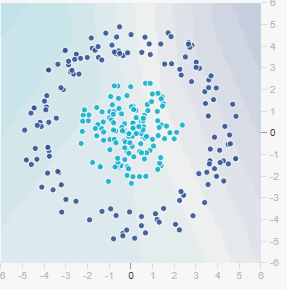
14.5 Visual Example: With 10% Training Data and Maximum Noise
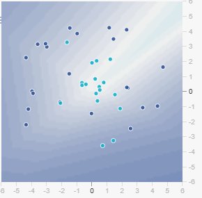
Figure: Training set with only 10% of data. Notice how sparse the samples are.
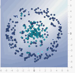
Figure: When you click “Show test data,” you see how extreme noise completely corrupts the circular pattern. The test set no longer follows a clear circle—it’s scattered chaos. The network cannot learn a robust boundary when the pattern itself is destroyed by noise.
14.6 The Generalization Gap
This scenario illustrates the critical concept of the generalization gap: the difference between training loss and test loss.
Healthy training: Training loss and test loss both decrease together, staying close.
Overfitting: Training loss decreases while test loss plateaus or increases. The gap widens.
The extreme case: Massive training loss decrease with near-zero improvement in test loss. The network has learned nothing useful.
14.6.1 Factors Contributing to Generalization Failure
Small Training Set: With only 10% of data (50-100 examples), the model sees each example many times. Batch size becomes critical—if batch size is large relative to training set, updates are infrequent and noisy.
High Noise (~0.5): Labels are almost random. The true signal is buried under noise.
Large Batch Size: Fewer weight updates per epoch. With tiny training set, this means very few gradient signals. The model doesn’t learn efficiently from the limited data.
Capacity: Even a modest hidden layer can memorize patterns in 100 noisy examples if given enough updates (training time).
14.6.2 Solutions in Practice
When facing this scenario, practitioners use:
Regularization: L1/L2 penalties, dropout, or early stopping to prevent overfitting.
More Data: Collect additional clean examples to provide more signal.
Reduce Batch Size: More frequent updates help the model learn from limited data. Small batches add noise (good for generalization) and provide frequent gradient signals.
Reduce Model Capacity: Use fewer neurons if possible, though this is limited by problem complexity.
Data Augmentation: Create new training examples by transforming existing ones (rotation, scaling, etc.).
Data Cleaning: Reduce noise in labels through manual review or automated methods.
15 Summary and Key Lessons
15.1 What We’ve Learned
Simplicity First: The Gaussian dataset teaches us that linear models work perfectly for linearly separable problems. Don’t add hidden layers unless necessary.
Activation Functions are Essential: Without nonlinear activation functions, hidden layers add no power. Stacking linear layers is equivalent to a single linear transformation.
Feature Engineering vs. Learning: XOR can be solved with engineered features (x₁ × x₂) and a linear classifier, or with hidden layers and nonlinear activations. Hidden layers essentially learn these features automatically.
ReLU is the Modern Standard: ReLU converges faster than Sigmoid or Tanh because it avoids vanishing gradients. This is why it became the default activation in 2011.
Problem-Dependent Design: Use the simplest architecture that solves your problem. Gaussian needs no hidden layers; XOR needs nonlinearity (either engineered features or hidden layers with activation functions).
15.2 Key Formulas to Remember
Node computation: \[z = \sum w_i x_i + b\]
Activation: \[a = \sigma(z)\]
Loss function (Binary Cross-Entropy): \[L = -[y \log(\hat{y}) + (1-y) \log(1-\hat{y})]\]
Weight update (Gradient Descent): \[w_{\text{new}} = w_{\text{old}} - \alpha \frac{\partial L}{\partial w}\]
ReLU activation: \[\text{ReLU}(z) = \max(0, z)\]
Sigmoid activation: \[\sigma(z) = \frac{1}{1 + e^{-z}}\]
15.3 Looking Ahead
In the next sections of Chapter 8, we’ll: - Implement neural networks from scratch in NumPy - Derive backpropagation in detail - Train on more complex datasets (MNIST handwritten digits) - Explore deeper networks and their challenges - Learn about regularization and optimization
- Replicate all questions in the TensorFlow Playground
- Record your observations for each configuration
- Verify the correct answers match your findings
- Explain in your own words why each architectural choice matters
- Experiment beyond the questions: Try learning rates in between (0.002, 0.005), different layer widths, etc.
This hands-on exploration builds intuition that will help you understand the mathematics in the coming sections.