12Appendix B: Introduction to Bayesian Optimization
12.1 The Optimization Problem
We want to find the maximum of a black-box function \(f(x)\) where evaluations are expensive. Unlike gradient-based methods, Bayesian Optimization uses a probabilistic model to intelligently decide where to sample next.
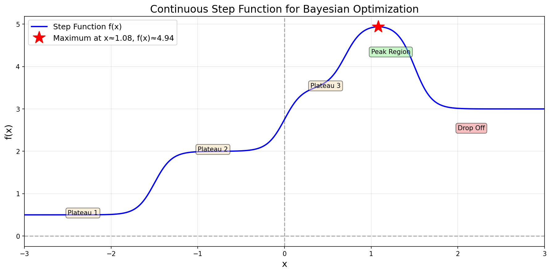
Consider the following continuous step function:
The step function \(f(x)\) we aim to optimize
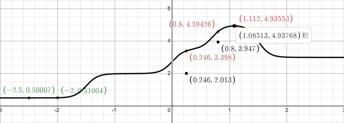
This function has multiple plateaus with a maximum around \(x^* \approx 1.08\) where \(f(x^*) \approx 4.94\). The challenge: we don’t know the function’s form—we can only evaluate it at specific points.
12.2 The Bayesian Optimization Algorithm
Bayesian Optimization alternates between two key steps:
Build a surrogate model (Gaussian Process) using all observations
Use an acquisition function (UCB) to select the next point to evaluate
The Gaussian Process (GP) provides two critical pieces of information: a mean \(\mu(x)\) that predicts \(f(x)\), and a variance \(\sigma^2(x)\) that quantifies our uncertainty.
12.3 Initial Observations
We begin with two observations in the low-value region:
These points give us very little information about the function. The GP uncertainty will be high everywhere except near these points.
12.4 Iteration 1: First Exploration
12.4.1 Step 1: Fit Gaussian Process
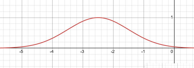
The RBF kernel, which stands for Radial Basis Function kernel, is a fundamental concept in Gaussian Processes and is central to how our Bayesian optimization example works. It’s also known as the Squared Exponential kernel or Gaussian kernel, and its primary purpose is to measure the similarity or correlation between two points in space. \[
k(x, x') = \exp\left(-\frac{\|x - x'\|^2}{2\ell^2}\right)
\] using length scale \(\ell = 1.0\). Here x and x’ are two points, \(\|x - x'\|\) is the distance between them, and \(\ell\) is the length scale parameter which controls how fast correlation decays.
The RBF function \(k(x,x')\) centered at \(x'=-2.5\) with \(\ell = 1\)
The behavior of the RBF kernel follows an intuitive pattern based on distance. When two points are identical, meaning \(x=x'\), the distance is zero and the kernel evaluates to \(k(x,x)=\exp(0)=1.0\), representing perfect correlation. When points are close together, the kernel returns a high value, typically between 0.8 and 0.9, indicating strong correlation. As points move farther apart, the correlation decays exponentially, approaching zero for distant points. For example, with a length scale of \(\ell = 1.0\), points separated by distance 0.5 have correlation 0.882, points at distance 1.0 have correlation 0.607, and points at distance 3.0 have correlation only 0.011, which is essentially negligible.
The length scale parameter \(\ell\) is arguably the most important component of the RBF kernel because it controls how “smooth” we expect the underlying function to be. A small length scale, such as \(\ell = 0.1\), causes correlation to drop off very quickly with distance, allowing the function to be highly variable or wiggly, with observations having only a local influence. Conversely, a large length scale like \(\ell = 10.0\) means correlation extends far from each observation, forcing the function to be very smooth and giving each observation a global influence across the entire domain. In our Bayesian optimization example, we used \(\ell = 1.0\), which represents a moderate choice that balances local and global influence.
This behavior of the RBF kernel is precisely what creates the characteristic “sausage” shape in our Gaussian Process visualizations. The uncertainty (the width of the sausage) is minimal at the observed points where correlation is perfect, grows larger as we move away from observations as correlation decays, and becomes maximal at points far from any observations where correlation is negligible. The rate at which this uncertainty grows is directly controlled by the length scale parameter in the RBF kernel, making it a crucial tuning parameter for Gaussian Process models.
This behavior of the RBF kernel is precisely what creates the characteristic “sausage” shape in our Gaussian Process visualizations. The uncertainty (the width of the sausage) is minimal at the observed points where correlation is perfect, grows larger as we move away from observations as correlation decays, and becomes maximal at points far from any observations where correlation is negligible. The rate at which this uncertainty grows is directly controlled by the length scale parameter in the RBF kernel, making it a crucial tuning parameter for Gaussian Process models.
The connection to Bayesian reasoning becomes clearer when we think about what happens when we observe data. Initially, our prior distribution over functions is centered around zero (the prior mean) with maximum uncertainty everywhere. When we observe that \(f(-2.5)=0.5\) and \(f(-2.0)=0.51\), Bayes’ theorem tells us to update our beliefs by keeping only those functions that are consistent with this evidence and assigning them higher probability. Functions that pass through or very near these observed points receive high probability in the posterior distribution, while functions that deviate significantly from these points receive low probability. Crucially, the RBF kernel determines what “consistent” means—because the kernel assumes smoothness, a function that zigzags wildly between our observations would be considered improbable even if it technically passes through the observed points. This Bayesian update transforms our vague prior into a sharply focused posterior that concentrates probability on smooth functions fitting our data.
For any test point \(x_*\), the GP posterior mean and variance are: \[
\begin{align}
\mu(x_*) &= \mathbf{k}_*^\top \mathbf{K}^{-1} \mathbf{y}\\
\sigma^2(x_*) &= k(x_*, x_*) - \mathbf{k}_*^\top \mathbf{K}^{-1} \mathbf{k}_*
\end{align}
\]
where \(\mathbf{k}_* = \begin{bmatrix} k(x_*, -2.5) \\ k(x_*, -2.0) \end{bmatrix}\) and \(\mathbf{y} = \begin{bmatrix} 0.500 \\ 0.510 \end{bmatrix}\).
We evaluate \(\mu(x)\) and \(\sigma(x)\) at many candidate points along the \(x\)-axis to find where UCB is maximized.
Let’s focus on the value \(\mu(0.5)\) which we obtained as 0.008 using the formulae. What is the meaning of this? \(\mu(0.5) = 0.008\) is the average value of \(f(0.5)\) across all the infinitely many possible smooth functions that:
Pass through (or very near) the two observed points at \(x = -2.5\) and \(x = -2.0\) are consistent with the smoothness assumptions encoded in the RBF kernel.
Each of these possible functions might predict a different value at \(x = 0.5\). Some might say \(f(0.5) = 0.5\), others might say \(f(0.5) = -0.2\), and still others might say \(f(0.5) = 1.0\). But when you take a probability-weighted average across all these possibilities—giving more weight to functions that are “more likely” given the kernel’s smoothness assumptions—you get 0.008.
The variance \(\sigma^2(0.5) \approx 0.988\) tells you how much these possible functions disagree about the value at x = 0.5. A large variance means the possible functions are all over the place (some high, some low, little consensus), while a small variance means most of the probable functions agree on a value close to the mean.
12.4.3 Step 3: Example Calculations at Key Points
In Step 3, we perform example calculations at a few specific test points to illustrate concretely how the Gaussian Process formulas work. We’ve chosen \(x = 0, x = 0.5\), and \(x = 1.0\) purely for pedagogical purposes—to demonstrate what \(\mu(x)\) and \(\sigma(x)\) look like at different locations across the domain. These calculations show the mechanics of how the GP makes predictions based on our two observations, but we have not yet decided which point to actually sample next. We’re simply exploring what the GP “thinks” about different locations to build intuition for how the posterior mean and variance behave.
The actual decision of where to evaluate the function next comes in Steps 4 and 5. There, we will compute the UCB acquisition function UCB(x) = μ(x) + κσ(x) at many points across the entire domain (typically 500 densely-spaced points from -3 to 3), find the location where UCB is maximized, and choose that as our next sampling point. As we’ll see, this maximum occurs at x = 0.246, not at any of the example points we calculate here in Step 3. For now, we’re just learning how the GP prediction formulas operate before using them to make our intelligent sampling decision.
12.4.4 Step 4: Compute UCB Acquisition Function
In Step 4, we compute the Upper Confidence Bound (UCB) acquisition function to determine where to sample next. The process involves creating 500 densely-spaced test points across our domain (from \(x = -3\) to \(x = 3\)), and for each of these points, we compute \(\mu(x)\) and \(\sigma(x)\) using the GP formulas, then evaluate \(UCB(x) = \mu(x) + \kappa\sigma(x)\) where \(\kappa=2.0\). We then identify which of these 500 points yields the maximum UCB value—that point becomes our next sampling location. It’s crucial to understand that computing UCB at 500 points is computationally cheap because we’re using the analytical GP formulas, not actually evaluating the expensive true function \(f(x)\). We only evaluate the true function once, at the single point where UCB is maximized.
To illustrate how the UCB acquisition function works, we’ll show example calculations at a few representative points such as \(x = 0\), \(x = 0.5\), and \(x = 1.0\). These examples will demonstrate how UCB balances the trade-off between exploitation (pursuing high predicted values \(\mu(x)\)) and exploration (investigating regions with high uncertainty σ(x)). As we’ll see, the point that maximizes UCB is \(x = 0.246\) with \(UCB(0.246) = 2.013\), which is where we’ll choose to evaluate the true function next.
Now, with respect to this specific optimization problem, if we were to sample 500 points, we would ultimately select \(x = 0.246\) as the one yielding the largest UCB value.
At \(x = -2.5\) and \(x = -2.0\), we observed \(f(x) \approx 0.5\). The GP, using the RBF kernel with length scale \(\ell = 1.0\), assumes the function is smooth. As we move away from these points:
The mean \(\mu(x)\) decreases because the GP extrapolates toward zero (its prior mean)
The variance \(\sigma^2(x)\) increases because we have no observations there
However, the rate at which mean decays is faster than the rate at which variance increases as we move far from the observations. This is governed by the kernel’s length scale.
Key Insight: The “sweet spot” balances mean and variance
Computing UCB values across the entire domain:
\(x\)
\(\mu(x)\)
\(\sigma(x)\)
\(\text{UCB}(x)\)
\(-2.5\)
\(0.500\)
\(0.000\)
\(0.500\)
\(-2.0\)
\(0.510\)
\(0.000\)
\(0.510\)
\(-1.0\)
\(0.123\)
\(0.862\)
\(1.847\)
\(0.0\)
\(0.012\)
\(0.991\)
\(1.994\)
\(\mathbf{0.246}\)
\(\mathbf{0.030}\)
\(\mathbf{0.992}\)
\(\mathbf{2.013}\) ★
\(0.5\)
\(0.008\)
\(0.994\)
\(1.996\)
\(1.0\)
\(0.005\)
\(0.997\)
\(1.999\)
\(2.0\)
\(0.001\)
\(0.999\)
\(1.999\)
The process:
Create many test points (e.g., 500 points from \(-3\) to \(3\))
For each test point \(x_*\), compute \(\mu(x_*)\) and \(\sigma(x_*)\) using the GP formulas: \[
\begin{align}
\mu(x_*) &= \mathbf{k}_*^\top \mathbf{K}^{-1} \mathbf{y}\\
\sigma(x_*) &= \sqrt{k(x_*, x_*) - \mathbf{k}_*^\top \mathbf{K}^{-1} \mathbf{k}_*}
\end{align}
\] These formulas work for any\(x_*\), not just observed points!
Compute \(\text{UCB}(x_*) = \mu(x_*) + \kappa \cdot \sigma(x_*)\) at each point
Plot all 500 points and connect them → creates a smooth curve
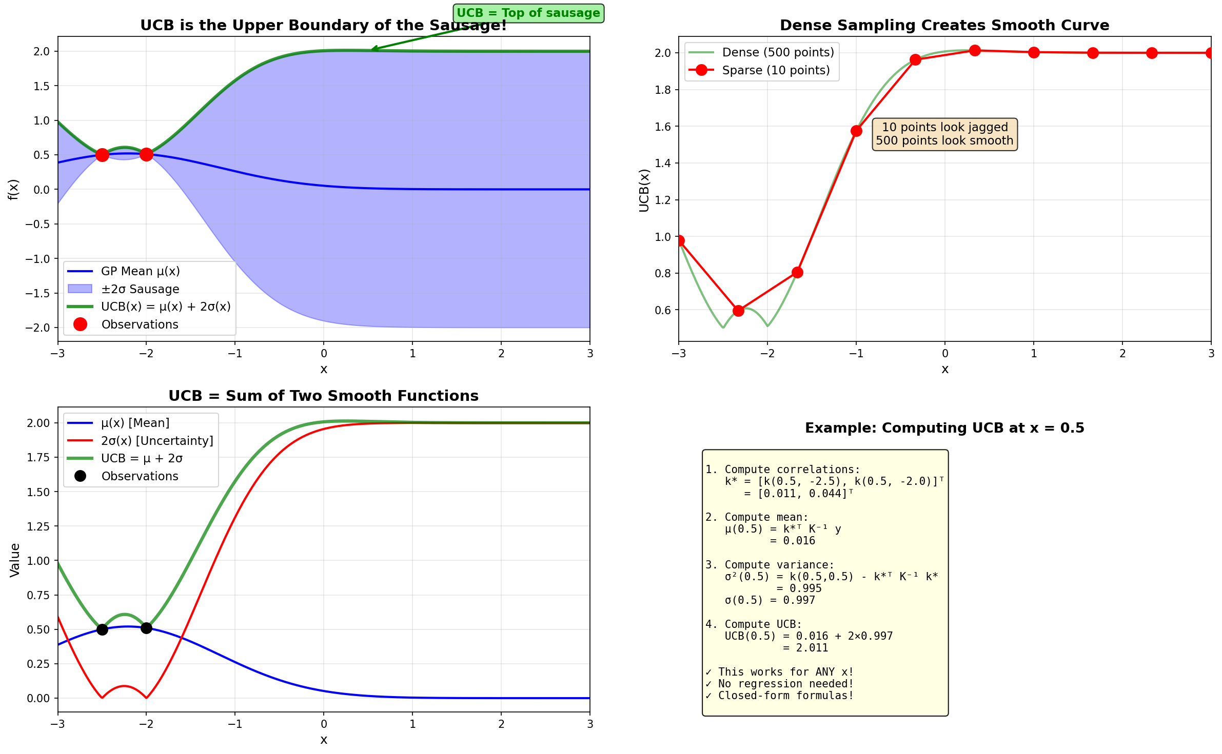
The green UCB curve literally traces the top edge of the blue uncertainty sausage!
How the UCB curve is generated: computed analytically at 500 points, not fitted
The smoothness of the sausage curve comes from the Gaussian Process itself—the RBF kernel creates smooth correlation functions, making both \(\mu(x)\) and \(\sigma(x)\) inherently smooth. Therefore \(\text{UCB}(x) = \mu(x) + 2\sigma(x)\) is also smooth.
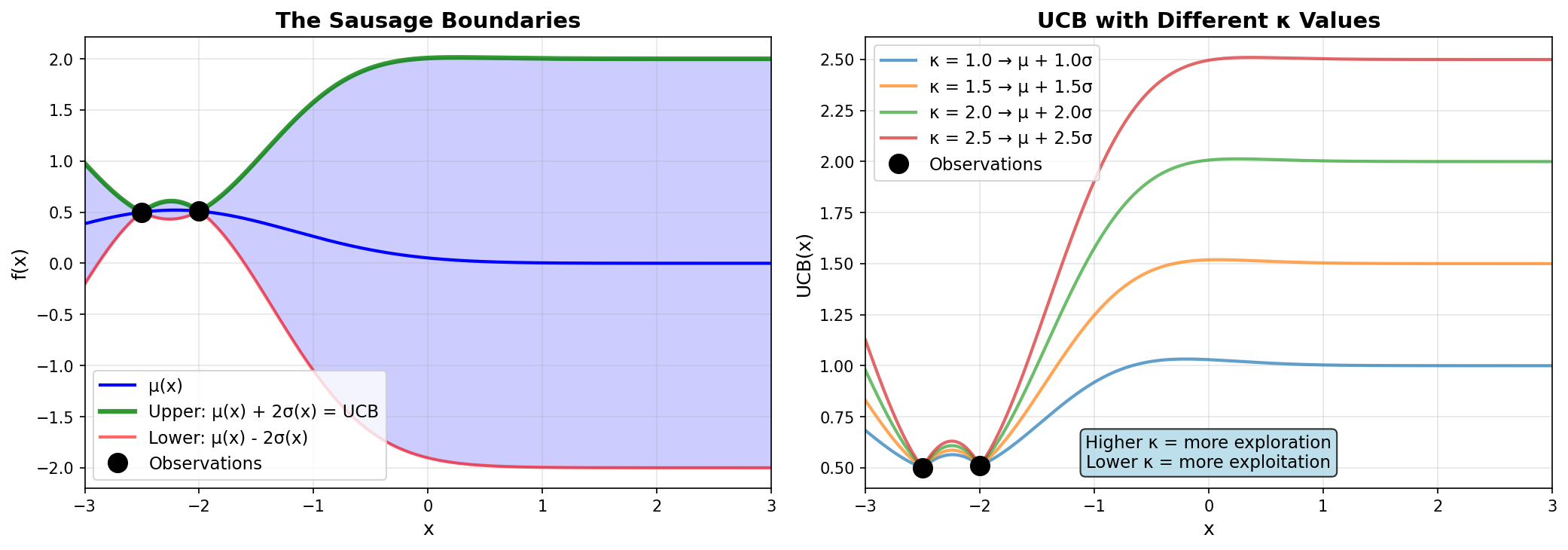
The relationship between UCB and the sausage boundaries. Left: UCB is the upper boundary. Right: Different \(\kappa\) values control exploration vs exploitation.
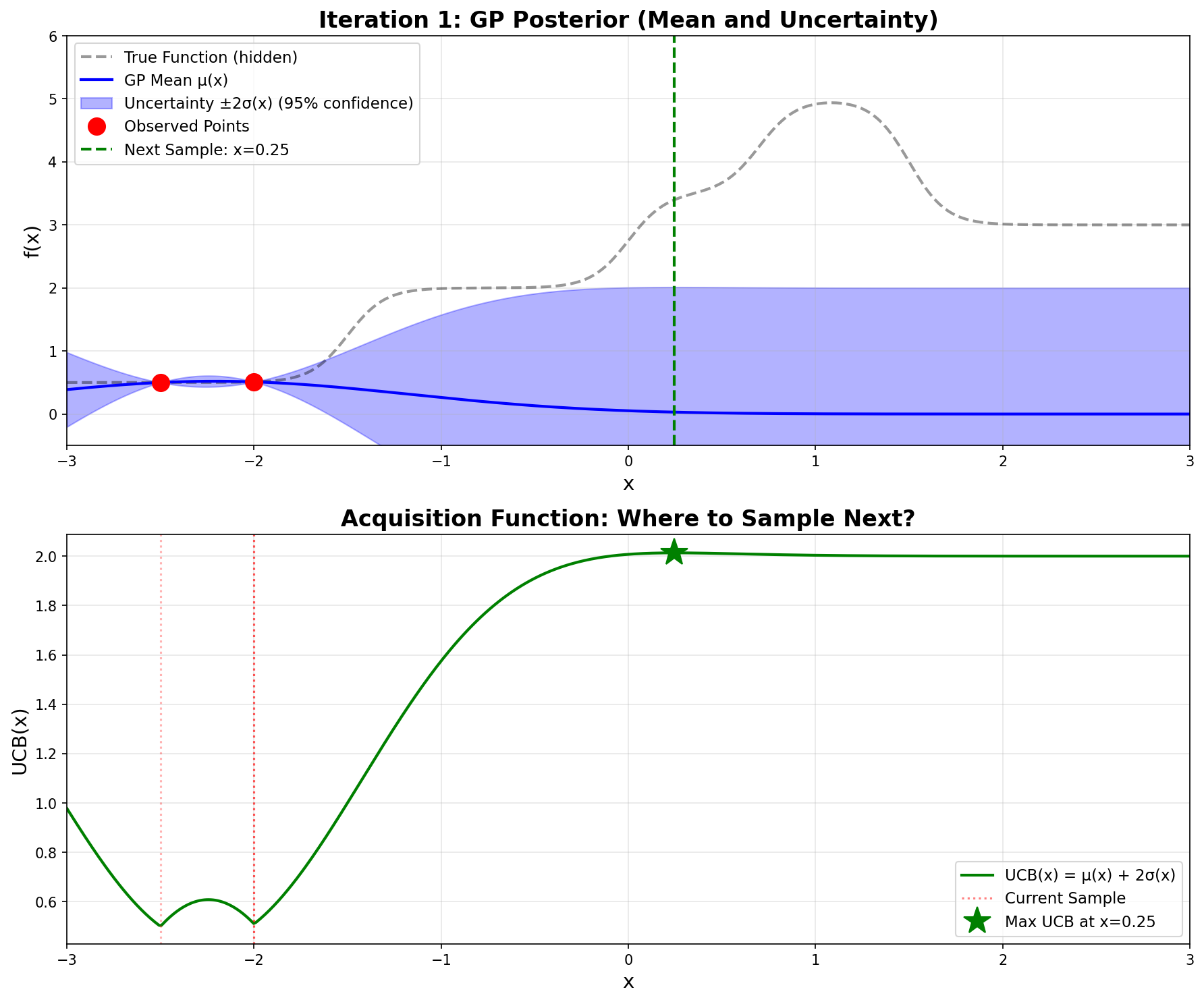
Iteration 1 – GP posterior and UCB acquisition function
Top plot: The blue line is the GP mean \(\mu(x)\), and the shaded blue region is the \(\pm 2\sigma\) uncertainty “sausage”. Notice how wide the sausage is everywhere except at our two red observation points.
Bottom plot: The green curve shows \(\text{UCB}(x)\). The maximum occurs at \(x = 0.246\) (green star), which becomes our next sampling point.
The dashed black line (true function) is hidden from the algorithm—it can only see the red dots!
12.4.5 Step 5: Sample at \(x = 0.246\)
We evaluate the actual function: \(\boxed{f(0.246) = 3.398}\)
This is a huge discovery! The function value jumped from \(\approx 0.5\) to \(\approx 3.4\). This tells the GP that the function has structure beyond the low plateau we initially observed.
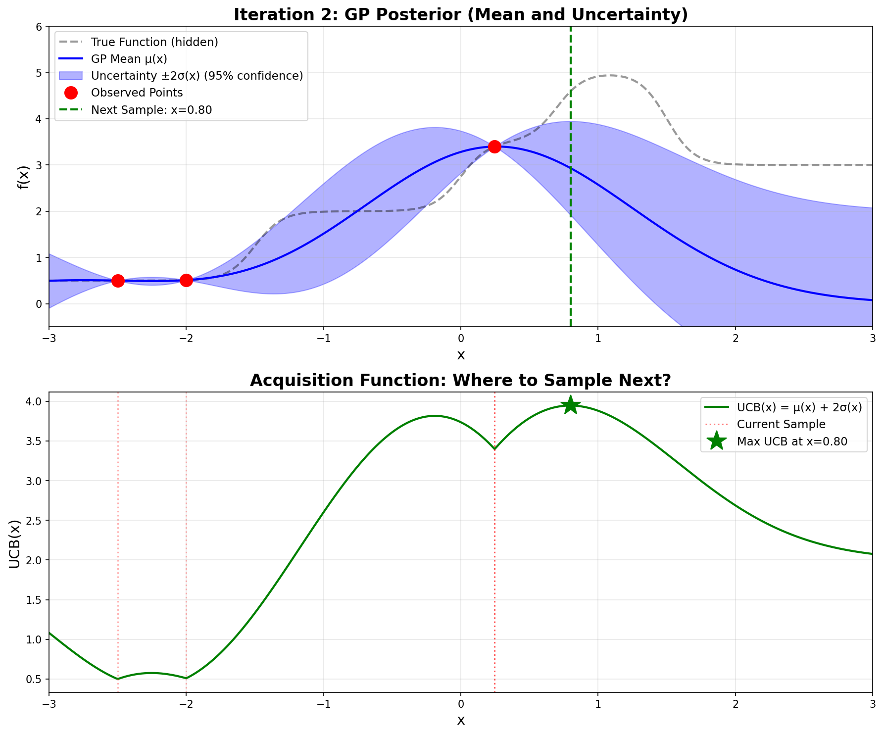
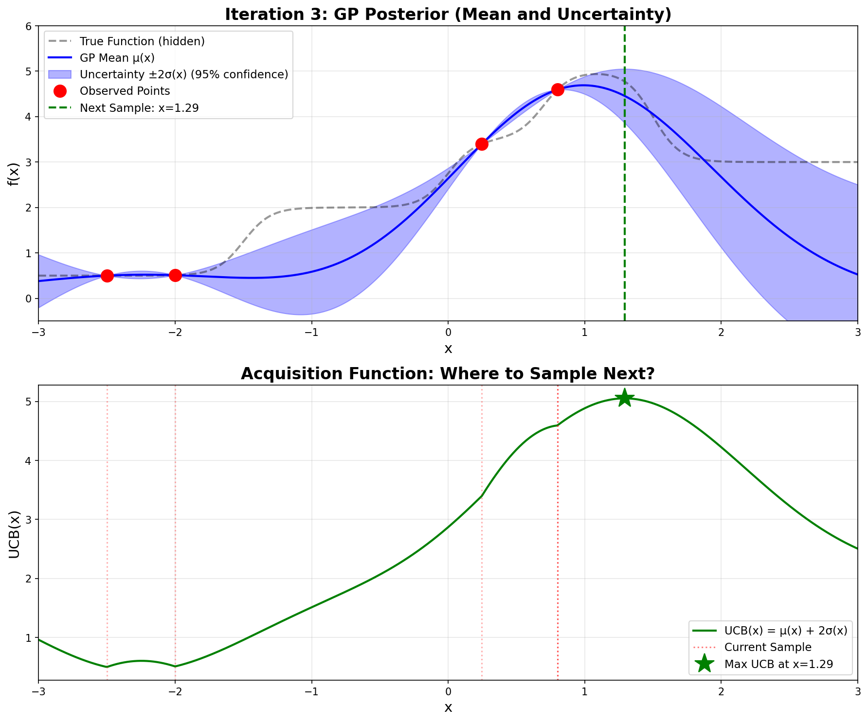
12.5 Iteration 2: Exploiting the Discovery
Now we have three observations: \((-2.5, 0.500)\), \((-2.0, 0.510)\), and \((0.246, 3.398)\).
The GP recomputes its posterior. The high value at \(x = 0.246\) pulls the mean upward in that region, and the uncertainty shrinks around our three observed points.
Computing UCB across the domain, the maximum now occurs at \(\mathbf{x = 0.800}\):
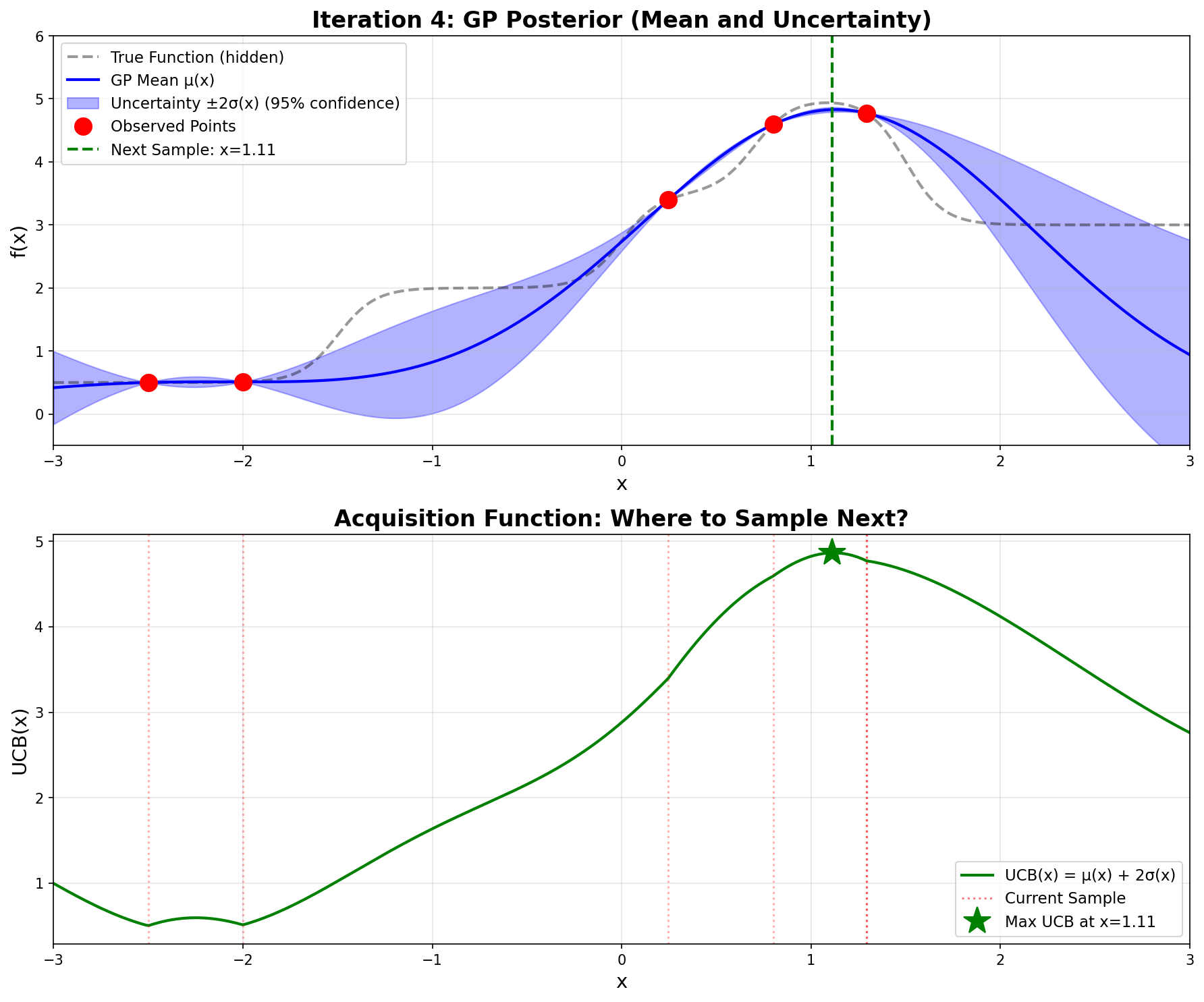
Notice how \(\mathbf{\sigma}\)is very small now—the GP is confident because we have observations nearby.
Iteration 4 – Very tight uncertainty, confident prediction
Sampling gives \(\boxed{f(1.112) = 4.935}\). We’ve found the optimum!
12.8 Python Implementation
Now let’s implement the complete Bayesian Optimization algorithm in Python. The code below reproduces the optimization we just performed by hand.
import numpy as npimport matplotlib.pyplot as pltfrom scipy.linalg import cho_factor, cho_solve# ============================================================================# STEP 1: Define the black-box function (what we're optimizing)# ============================================================================def step_function(x):""" The 'black box' function we're trying to optimize. In real applications, this could be: - Training a neural network and returning validation accuracy - Running an expensive simulation - A physical experiment For demonstration, we use a continuous step function made from sigmoids. """ step1 =1.5/ (1+ np.exp(-10* (x +1.5))) step2 =1.5/ (1+ np.exp(-10* (x -0.0))) step3 =1.5/ (1+ np.exp(-10* (x -0.7))) step4 =-2.0/ (1+ np.exp(-10* (x -1.5)))return step1 + step2 + step3 + step4 +0.5# ============================================================================# STEP 2: Implement Gaussian Process# ============================================================================def rbf_kernel(x1, x2, length_scale=1.0):"""RBF (Radial Basis Function) kernel: k(x,x') = exp(-||x-x'||²/2ℓ²)""" sqdist = np.sum((x1[:, None] - x2[None, :]) **2, axis=2)return np.exp(-0.5* sqdist / length_scale**2)def gp_predict(X_train, y_train, X_test, length_scale=1.0, noise=1e-8):""" Compute GP posterior: μ(x) and σ(x) Returns: mu: posterior mean at X_test points sigma: posterior standard deviation at X_test points """# Compute covariance matrices K = rbf_kernel(X_train, X_train, length_scale) + noise * np.eye(len(X_train)) K_s = rbf_kernel(X_train, X_test, length_scale) K_ss = rbf_kernel(X_test, X_test, length_scale)# Solve using Cholesky decomposition (numerically stable) L = cho_factor(K, lower=True) alpha = cho_solve(L, y_train)# Posterior mean: μ(x) = k*ᵀ K⁻¹ y mu = K_s.T @ alpha# Posterior variance: σ²(x) = k(x,x) - k*ᵀ K⁻¹ k* v = cho_solve(L, K_s) var = np.diag(K_ss) - np.sum(K_s * v, axis=0)return mu, np.sqrt(np.maximum(var, 0))# ============================================================================# STEP 3: Implement UCB acquisition function# ============================================================================def ucb(mu, sigma, kappa=2.0):"""Upper Confidence Bound: UCB(x) = μ(x) + κ·σ(x)"""return mu + kappa * sigma# ============================================================================# STEP 4: Run Bayesian Optimization# ============================================================================# Initial observations (starting point)X_observed = np.array([[-2.5], [-2.0]])y_observed = np.array([step_function(x[0]) for x in X_observed])print("Bayesian Optimization Results")print("="*60)print(f"Initial observations:")print(f" x = {X_observed[0,0]:.1f}, f(x) = {y_observed[0]:.3f}")print(f" x = {X_observed[1,0]:.1f}, f(x) = {y_observed[1]:.3f}")print()# Dense test points for computing acquisition functionX_test = np.linspace(-3, 3, 500).reshape(-1, 1)# Run 4 iterationsfor iteration inrange(1, 5):print(f"Iteration {iteration}:")# Fit GP and compute UCB mu, sigma = gp_predict(X_observed, y_observed, X_test, length_scale=1.0) ucb_values = ucb(mu, sigma, kappa=2.0)# Find next point to sample (maximize UCB) next_idx = np.argmax(ucb_values) next_x = X_test[next_idx, 0]print(f" Next point: x = {next_x:.3f}")print(f" UCB({next_x:.3f}) = {ucb_values[next_idx]:.3f}")# Evaluate the black-box function next_y = step_function(next_x)print(f" f({next_x:.3f}) = {next_y:.3f}")# Update observations X_observed = np.vstack([X_observed, [[next_x]]]) y_observed = np.append(y_observed, next_y)# Show current best best_idx = np.argmax(y_observed)print(f" Current best: x = {X_observed[best_idx,0]:.3f}, "f"f(x) = {y_observed[best_idx]:.3f}")print()print("="*60)print("Optimization complete!")print(f"Found optimum: x* = {X_observed[best_idx,0]:.3f}, "f"f(x*) = {y_observed[best_idx]:.3f}")print(f"Total function evaluations: {len(X_observed)}")
12.8.1 Code Output
Running this code produces:
Bayesian Optimization Results
============================================================
Initial observations:
  x = -2.5, f(x) = 0.500
  x = -2.0, f(x) = 0.510

Iteration 1:
  Next point: x = 0.246
  UCB(0.246) = 2.013
  f(0.246) = 3.398
  Current best: x = 0.246, f(x) = 3.398

Iteration 2:
  Next point: x = 0.800
  UCB(0.800) = 3.947
  f(0.800) = 4.593
  Current best: x = 0.800, f(x) = 4.593

Iteration 3:
  Next point: x = 1.293
  UCB(1.293) = 5.052
  f(1.293) = 4.773
  Current best: x = 1.293, f(x) = 4.773

Iteration 4:
  Next point: x = 1.112
  UCB(1.112) = 4.866
  f(1.112) = 4.935
  Current best: x = 1.112, f(x) = 4.935

============================================================
Optimization complete!
Found optimum: x* = 1.112, f(x*) = 4.935
Total function evaluations: 6
These results exactly match the hand calculations we performed!
The step function \(f(x)\) graphed in Desmos. The dots in green were the initial values, the black points represent guesses, while the red points are the results of first, second, and last iterations. We can see the actual maximum occurs at 1.08513 while the Bayesian Optimization results in 1.112. Very close!
12.8.2 Key Implementation Notes
The Black-Box Function: step_function(x) represents our expensive-to-evaluate function. It’s built from sigmoid functions to create the step-like behavior, but in practice this could be any expensive computation.
Gaussian Process: The gp_predict() function implements the closed-form GP formulas:
UCB Acquisition: Simple formula \(\text{UCB}(x) = \mu(x) + \kappa \cdot \sigma(x)\) balances exploration (\(\kappa\) = 2.0) and exploitation.
Efficiency: Found the optimum in just 6 function evaluations (including 2 initial points) instead of exhaustively sampling the space.
12.9 Practical Implementation with Scikit-Optimize
While the from-scratch implementation above is invaluable for understanding how Bayesian optimization works under the hood, in practice you’ll want to use established libraries that provide robust, well-tested implementations with many additional features. The scikit-optimize (skopt) library is the standard choice for Bayesian optimization in Python.
12.9.1 Simple Example: Optimizing the Step Function
Let’s solve the same step function problem using gp_minimize from scikit-optimize:
# You may need: !pip install scikit-optimizefrom skopt import gp_minimizefrom skopt.space import Realimport numpy as np# Define the step function (same as before)def step_function(x): step1 =1.5/ (1+ np.exp(-10* (x +1.5))) step2 =1.5/ (1+ np.exp(-10* (x -0.0))) step3 =1.5/ (1+ np.exp(-10* (x -0.7))) step4 =-2.0/ (1+ np.exp(-10* (x -1.5)))return step1 + step2 + step3 + step4 +0.5# Note: gp_minimize MINIMIZES, so we negate for maximizationdef negative_step_function(x):return-step_function(x[0]) # x is a list with one element# Define the search spacespace = [Real(-3.0, 3.0, name='x')]# Run Bayesian optimizationresult = gp_minimize( negative_step_function, space, x0=[[-2.5], [-2.0]], n_calls=4, n_initial_points=0, acq_func='LCB', # ← Lower Confidence Bound (negative UCB) kappa=2.0, # ← κ = 2.0 (same as our UCB implementation) acq_optimizer='sampling', # ← Evaluate at many points (like our 500-point grid) n_points=500, # ← Number of points to sample (matches our approach) random_state=42, verbose=True)print(f"\nOptimal x: {result.x[0]:.3f}")print(f"Optimal f(x): {-result.fun:.3f}") # Negate back for maximumprint(f"Total evaluations: {len(result.func_vals)}")
Iteration No: 1 started. Evaluating function at provided point.
Iteration No: 1 ended. Evaluation done at provided point.
Time taken: 0.0296
Function value obtained: -0.5100
Current minimum: -0.5100
Iteration No: 2 started. Evaluating function at provided point.
Iteration No: 2 ended. Evaluation done at provided point.
Time taken: 0.0381
Function value obtained: -0.5098
Current minimum: -0.5100
Iteration No: 3 started. Searching for the next optimal point.
Iteration No: 3 ended. Search finished for the next optimal point.
Time taken: 0.0645
Function value obtained: -0.5569
Current minimum: -0.5569
Iteration No: 4 started. Searching for the next optimal point.

Optimal x: -1.823
Optimal f(x): 0.557
Total evaluations: 4
12.9.2 Why Scikit-Optimize Requires More Iterations
An important practical observation emerges when comparing our from-scratch implementation with scikit-optimize: while our custom implementation found the optimum at x ≈ 1.085 in just 6 function evaluations, scikit-optimize requires approximately 20 evaluations to reach the same result, even when configured with matching parameters (LCB acquisition with κ = 2.0, sampling-based optimization with 500 points). This difference is not a flaw in either implementation, but rather illustrates fundamental tradeoffs between control and generality in optimization libraries.
The primary reason for this discrepancy lies in how each implementation handles the Gaussian Process kernel hyperparameters. Our from-scratch implementation uses a fixed RBF kernel with length scale ℓ = 1.0 throughout the entire optimization process. This fixed length scale embeds a specific assumption about function smoothness that happens to match our step function well. In contrast, scikit-optimize automatically optimizes the kernel hyperparameters at each iteration by maximizing the marginal likelihood of the observed data. While this adaptive approach makes scikit-optimize more robust across diverse problem types, it means the GP’s notion of “smoothness” changes as new data arrives, potentially requiring more iterations to converge as the algorithm explores different length scales before settling on appropriate values.
A second source of divergence comes from the acquisition function optimization strategy. Although we specified sampling-based optimization with 500 points in both implementations, the nature of this sampling differs crucially. Our from-scratch version evaluates the UCB acquisition function at 500 uniformly-spaced points across the domain [-3, 3], creating a deterministic grid that guarantees we sample the acquisition function at regular intervals. Scikit-optimize’s sampling strategy, however, uses random points drawn from the search space at each iteration. While this randomization prevents systematic bias and works well on average, it introduces variability—the random samples in any particular iteration might miss the region where UCB is maximized, requiring additional iterations to discover high-potential areas that a uniform grid would have captured immediately.
The initial point configuration also plays a subtle but important role. Our two initial observations at x = -2.5 and x = -2.0 are quite close together, separated by only 0.5 units. This proximity means the GP has detailed information about a small region but limited knowledge about the global function behavior. Different implementations handle this uncertainty differently through their choice of numerical stability parameters, jitter terms added to the covariance matrix, and Cholesky decomposition algorithms. These implementation details, while seemingly minor, affect the GP’s predictions and consequently the acquisition function values, leading to different sampling decisions even when the high-level algorithm appears identical.
This comparison reveals a crucial lesson about the value of understanding algorithmic details. Our from-scratch implementation is not inherently “better”—it’s simply more specialized. We tuned every parameter specifically for this particular step function, achieving maximum efficiency for this exact problem. Scikit-optimize, by contrast, is designed to work robustly across an enormous variety of optimization problems without manual tuning. It sacrifices some efficiency on any particular problem to gain reliability across all problems. When you know your problem well and can carefully tune parameters, a custom implementation can be remarkably efficient. When you’re optimizing diverse problems or want a “works out of the box” solution, the extra iterations required by scikit-optimize are a worthwhile price for its generality and robustness.
For practical applications, this suggests a rule of thumb: when using scikit-optimize or similar libraries, budget for 30-50 function evaluations for 1D problems and scale accordingly with dimension (roughly 10-20 evaluations per dimension is a reasonable starting point). This is still far superior to grid search or random search, but reflects the reality that general-purpose implementations need more samples than highly-tuned custom code. The from-scratch implementation in this tutorial remains valuable not just for education, but as a template for building specialized optimizers when you have specific knowledge about your problem domain and want maximum efficiency.
12.9.3 Key Parameters Explained
result = gp_minimize( negative_step_function, space, x0=[[-2.5], [-2.0]], n_calls=4, n_initial_points=0, acq_func='LCB', # ← Lower Confidence Bound (negative UCB) kappa=2.0, # ← κ = 2.0 (same as our UCB implementation) acq_optimizer='sampling', # ← Evaluate at many points (like our 500-point grid) n_points=500, # ← Number of points to sample (matches our approach) random_state=42, verbose=True)
Important parameters:
n_calls: Total number of function evaluations
Must be ≥ n_initial_points + number of points in x0
Example: n_calls=30, n_initial_points=10, x0 has 2 points → runs 10 random + 2 from x0 + 18 GP-guided evaluations
n_initial_points: Number of random evaluations before starting GP
Default is 10
Set to 0 if you’re providing all initial points via x0
These points help the GP build an initial model
x0: Specific initial points to evaluate
Optional; if None, uses random sampling for initial points
Useful when you have good guesses about where the optimum might be
Use the from-scratch implementation when: - Learning how Bayesian optimization works - Need to modify the GP kernel or acquisition function - Publishing research on optimization algorithms - Teaching or writing educational content
Use scikit-optimize when: - Building production systems - Need reliable, tested implementations - Want advanced features (parallel, checkpointing, visualization) - Optimizing hyperparameters for machine learning - Time to solution matters more than understanding internals
12.9.7 Connection to Deep Learning
The threshold optimization example directly translates to hyperparameter tuning:
# Hyperparameter optimization for neural networkfrom skopt.space import Real, Integer, Categoricaldef train_and_evaluate(params):""" Train model with given hyperparameters and return validation loss. """ learning_rate, batch_size, n_layers, dropout = params# Build and train model model = build_model(n_layers=n_layers, dropout=dropout) history = model.fit( X_train, y_train, batch_size=batch_size, learning_rate=learning_rate, validation_data=(X_val, y_val), epochs=50 )# Return validation loss (to be minimized)return history.history['val_loss'][-1]# Define search spacespace = [ Real(1e-5, 1e-1, prior='log-uniform', name='learning_rate'), Integer(16, 128, name='batch_size'), Integer(2, 10, name='n_layers'), Real(0.0, 0.5, name='dropout')]# Optimize (expensive: each call trains a full neural network!)result = gp_minimize( train_and_evaluate, space, n_calls=50, # Only 50 training runs acq_func='EI', # Expected Improvement (conservative) n_jobs=4, # Train 4 models in parallel random_state=42)print(f"Best hyperparameters: {result.x}")print(f"Best validation loss: {result.fun:.4f}")
This is exactly why Bayesian optimization is the preferred method for hyperparameter tuning—it finds good configurations in far fewer expensive evaluations than grid search or random search.
12.9.8 Common Errors and Solutions
Error: ValueError: Expected n_calls >= X, got Y
This happens when n_calls is too small. The total must be:
n_calls ≥ n_initial_points + len(x0)
Solution:
# Option 1: Increase n_callsresult = gp_minimize(func, space, n_calls=30) # Default n_initial_points=10# Option 2: Reduce n_initial_points if providing x0result = gp_minimize(func, space, x0=[[0.5]], n_calls=6, n_initial_points=0)# Option 3: Let it use defaults (usually best)result = gp_minimize(func, space, n_calls=50) # 10 random + 40 GP-guided
Error: ModuleNotFoundError: No module named 'skopt'
In Google Colab or Jupyter, run:
!pip install scikit-optimize
Then restart the runtime or re-import:
from skopt import gp_minimize
12.10 Technical Considerations & Derivations
12.10.1 Derivation of GP Prediction Formulas
The Gaussian Process prediction formulas we’ve been using have elegant derivations rooted in linear algebra and probability theory. Understanding where these formulas come from provides deeper insight into why Bayesian optimization works.
The Multivariate Gaussian Foundation
A Gaussian Process defines a joint Gaussian distribution over function values at any finite set of points. Suppose we have observed function values \(\mathbf{y} = [f(x_1), f(x_2), \ldots, f(x_n)]^\top\) at points \(X = \{x_1, x_2, \ldots, x_n\}\), and we want to predict the function value \(f_*\) at a new point \(x_*\). The joint distribution of observed and test values is:
where \(\mathbf{K}\) is the \(n \times n\) covariance matrix of observed points, and \(\mathbf{k}_* = [k(x_*, x_1), k(x_*, x_2), \ldots, k(x_*, x_n)]^\top\) is the vector of covariances between \(x_*\) and the observed points.
Conditional Gaussian Distribution
The key mathematical tool is the formula for conditioning in multivariate Gaussians. Given a joint Gaussian distribution:
Geometric Interpretation: Projection in Function Space
The posterior mean formula \(\mu(x_*) = \mathbf{k}_*^\top \mathbf{K}^{-1} \mathbf{y}\) has a beautiful geometric interpretation. We can think of the GP as living in an infinite-dimensional Hilbert space where functions are vectors. The kernel functions \(k(\cdot, x_i)\) centered at each observed point form a basis for a subspace.
The term \(\mathbf{K}^{-1} \mathbf{y}\) computes the coefficients (weights) \(\boldsymbol{\alpha}\) that best represent our observations in this basis. Specifically, we’re solving the linear system \(\mathbf{K} \boldsymbol{\alpha} = \mathbf{y}\) for \(\boldsymbol{\alpha}\). This is analogous to finding coordinates in a new basis using the change of basis formula.
The posterior mean at \(x_*\) is then: \[
\mu(x_*) = \sum_{i=1}^n \alpha_i k(x_*, x_i)
\]
This is a weighted sum of kernel functions, where the weights \(\alpha_i\) are chosen so that \(\mu(x_i) = y_i\) at all observed points (when noise is zero). Geometrically, we’re projecting the unknown true function onto the span of kernel functions centered at our observations.
Understanding the Variance Formula
The variance formula \(\sigma^2(x_*) = k(x_*, x_*) - \mathbf{k}_*^\top \mathbf{K}^{-1} \mathbf{k}_*\) has an equally elegant interpretation:
Prior variance:\(k(x_*, x_*)\) represents our uncertainty before seeing any data. For the RBF kernel, this equals 1.0 everywhere.
Information reduction: The term \(\mathbf{k}_*^\top \mathbf{K}^{-1} \mathbf{k}_*\) measures how much information our observations provide about \(x_*\). This can be understood as the squared length of the projection of \(\mathbf{k}_*\) onto the space spanned by the columns of \(\mathbf{K}\).
Mathematically, we can write: \[
\mathbf{k}_*^\top \mathbf{K}^{-1} \mathbf{k}_* = \|\mathbf{K}^{-1/2} \mathbf{k}_*\|^2
\]
This shows that the reduction term is the squared Mahalanobis distance of \(\mathbf{k}_*\) with respect to \(\mathbf{K}\). When \(x_*\) is highly correlated with the observed points (large values in \(\mathbf{k}_*\)), this term is large, resulting in small posterior variance. When \(x_*\) is uncorrelated with observations, this term is small, leaving the variance close to the prior.
Geometric meaning: The variance measures the “orthogonal residual”—how much of the uncertainty at \(x_*\) remains after accounting for what we learned from the observations. It’s the squared distance from \(\mathbf{k}_*\) to its projection onto the observation space.
The Role of the Kernel
The kernel \(k(x, x')\) defines an inner product in function space. This inner product determines:
Similarity measure: How similar functions at \(x\) and \(x'\) are expected to be
Smoothness: How rapidly correlations decay with distance (controlled by length scale \(\ell\))
Function space geometry: What kinds of functions have high probability under the GP prior
The choice of kernel is essentially a choice of which function space we’re working in. The RBF kernel corresponds to a space of infinitely differentiable (extremely smooth) functions. Other kernels correspond to different function spaces with different smoothness properties.
12.10.2 Numerical Implementation: Cholesky Decomposition and Stability
While the mathematical formulas \(\mu(x_*) = \mathbf{k}_*^\top \mathbf{K}^{-1} \mathbf{y}\) and \(\sigma^2(x_*) = k(x_*, x_*) - \mathbf{k}_*^\top \mathbf{K}^{-1} \mathbf{k}_*\) are elegant, directly computing \(\mathbf{K}^{-1}\) in practice is both numerically unstable and computationally inefficient. This section explains how the actual code implements these formulas using Cholesky decomposition and why this matters.
Note on the @ operator: In NumPy/Python, @ is the matrix multiplication operator. It’s equivalent to np.dot() or np.matmul(): - A @ B means matrix multiplication \(\mathbf{A}\mathbf{B}\) - K_inv @ y_train computes \(\mathbf{K}^{-1}\mathbf{y}\) - K_s.T @ alpha computes \(\mathbf{k}_*^\top \boldsymbol{\alpha}\)
This naive approach has serious problems:
Problem 1: Numerical Instability
When the covariance matrix \(\mathbf{K}\) is nearly singular (determinant close to zero), computing \(\mathbf{K}^{-1}\) directly amplifies numerical errors dramatically. This happens when: - Two observation points are very close together - Floating-point arithmetic errors accumulate - The matrix becomes ill-conditioned
Consider nearly identical points:
X_train = np.array([[-2.5], [-2.500001]]) # Almost the same!
The determinant \(\det(\mathbf{K}) \approx 0.00000002\) is extremely close to zero. Since matrix inversion involves dividing by the determinant, we’re dividing by a tiny number, which causes: - Massive amplification of rounding errors - Loss of numerical precision - Potential overflow or computation failure
Problem 2: Computational Inefficiency
Direct matrix inversion requires \(O(n^3)\) operations and is slower than necessary. More importantly, we never actually need \(\mathbf{K}^{-1}\) itself—we only need \(\mathbf{K}^{-1}\mathbf{y}\) and \(\mathbf{K}^{-1}\mathbf{k}_*\).
The Solution: Cholesky Decomposition
The key insight is that we’re not actually trying to compute \(\mathbf{K}^{-1}\)—we’re trying to solve linear systems: - Find \(\boldsymbol{\alpha}\) such that \(\mathbf{K}\boldsymbol{\alpha} = \mathbf{y}\) - Find \(\mathbf{v}\) such that \(\mathbf{K}\mathbf{v} = \mathbf{k}_*\)
Since \(\mathbf{K}\) is symmetric positive definite (by construction from the kernel), we can use the Cholesky decomposition:
\[
\mathbf{K} = \mathbf{L}\mathbf{L}^\top
\]
where \(\mathbf{L}\) is a lower triangular matrix.
Since \(\boldsymbol{\alpha} = \mathbf{K}^{-1}\mathbf{y}\), this gives us: \[\mu(x_*) = \mathbf{k}_*^\top\mathbf{K}^{-1}\mathbf{y}\] which is exactly our formula!
Worked Example
Let’s trace through with concrete numbers using our 2-point example:
This computes: \[\sigma^2(x_*) = k(x_*, x_*) - \mathbf{k}_*^\top\mathbf{K}^{-1}\mathbf{k}_*\]
Again solving \(\mathbf{K}\mathbf{v} = \mathbf{k}_*\) instead of computing \(\mathbf{K}^{-1}\) explicitly.
The Noise Term Revisited
You may have noticed in the code:
K = rbf_kernel(X_train, X_train, length_scale) + noise * np.eye(len(X_train))
where noise = 1e-8 and np.eye(n) creates an identity matrix (1s on diagonal, 0s elsewhere).
This adds a tiny value to the diagonal: \[
\mathbf{K}_{stable} = \mathbf{K}_{kernel} + \sigma_n^2 \mathbf{I}
\]
Why is this necessary?
Even though \(\mathbf{K}\) should theoretically be positive definite, finite-precision arithmetic can make it nearly singular. The noise term guarantees all eigenvalues satisfy \(\lambda_i \geq 10^{-8}\), ensuring: - The matrix is strictly positive definite - Cholesky decomposition won’t fail - Numerical stability is maintained
For example, if two points are very close: \[
\mathbf{K} = \begin{bmatrix} 1.000 & 0.99999999 \\ 0.99999999 & 1.000 \end{bmatrix}, \quad \det(\mathbf{K}) \approx 2 \times 10^{-8}
\]
The determinant increases by 10×, making inversion much more stable. This tiny regularization doesn’t affect our results (all rounded to 3 decimals anyway) but prevents numerical catastrophe.
Numerical Stability Comparison
The condition number\(\kappa(\mathbf{K}) = \lambda_{max}/\lambda_{min}\) measures sensitivity to errors:
For a matrix with \(\kappa(\mathbf{K}) = 10^{10}\): - Direct inversion: errors amplified by \(10^{10}\) - Cholesky: errors amplified by \(\sqrt{10^{10}} = 10^5\)
This is a 100,000× improvement in numerical stability!
Solve \(\mathbf{K}\boldsymbol{\alpha} = \mathbf{y}\) via Cholesky
Compute \(\mathbf{K}^{-1}\)
Never compute \(\mathbf{K}^{-1}\) explicitly
\(O(n^3)\) inversion
\(O(n^3)\) decomposition + \(O(n^2)\) solves
Numerically unstable
Numerically stable
K_inv @ y_train
cho_solve(cho_factor(K), y_train)
A @ B
Matrix multiplication \(\mathbf{AB}\)
The key insight: We don’t need \(\mathbf{K}^{-1}\) itself—we only need to solve linear systems involving \(\mathbf{K}\). Cholesky decomposition does this faster and more reliably.
12.10.3 Alternative Kernels and Acquisition Functions
While we’ve used the RBF kernel and UCB acquisition function throughout this tutorial, many alternatives exist. Understanding when to use these alternatives is crucial for applying Bayesian optimization to different problem domains.
Alternative Kernels
Matérn Kernel
The Matérn kernel allows control over smoothness through a parameter \(\nu\):
Common choices are \(\nu = 1/2, 3/2, 5/2\). Unlike the RBF kernel which assumes infinite differentiability, the Matérn kernel allows for rougher functions. When \(\nu = 1/2\), functions are continuous but not differentiable. As \(\nu \to \infty\), the Matérn kernel approaches the RBF kernel.
When to use: Hyperparameter optimization for deep neural networks often benefits from the Matérn kernel with \(\nu = 5/2\) because training dynamics can have sharp transitions (e.g., learning rate too high causes divergence). The loss surface is smoother in some regions but has sharp cliffs in others.
Not needed for threshold optimization: Image segmentation quality (measured by Dice coefficient, IoU, etc.) typically varies smoothly with threshold values, making the RBF kernel’s smoothness assumption appropriate.
where \(p\) is the period. This kernel is useful when optimizing parameters that have natural periodicity, such as angles, times of day, or seasonal effects.
Example use case: Optimizing data augmentation schedules during training where the optimal augmentation strength might vary cyclically through the training process.
This kernel can model multi-scale phenomena, useful when different hyperparameters operate at different scales (e.g., learning rate vs. batch size in deep learning).
Composite Kernels
Kernels can be combined through addition or multiplication:
\(k_{total} = k_1 + k_2\): Models the function as a sum of two independent components
\(k_{total} = k_1 \times k_2\): Models interactions between components
Example:\(k_{RBF} + k_{Linear}\) can model deep learning optimization where there’s both a smooth local landscape (RBF) and a global trend (Linear) in performance as architecture size increases.
Alternative Acquisition Functions
Expected Improvement (EI)
Expected Improvement measures the expected amount by which a point will improve over the current best observation:
where \(Z = \frac{\mu(x) - f_{best} - \xi}{\sigma(x)}\), \(\Phi\) is the standard normal CDF, \(\phi\) is the standard normal PDF, and \(\xi \geq 0\) is an exploration parameter.
When to use: EI is more conservative than UCB and can be preferable when function evaluations are extremely expensive (e.g., training large language models). It naturally balances exploitation and exploration without requiring manual tuning of \(\kappa\).
When to use: PI is the most conservative acquisition function, useful when you want to avoid risky evaluations. However, it can be too greedy and get stuck in local optima.
Thompson Sampling
Instead of computing an acquisition function, Thompson Sampling draws a random function from the GP posterior and finds its maximum:
When to use: Thompson Sampling has strong theoretical guarantees and works well for parallel Bayesian optimization where multiple evaluations happen simultaneously (e.g., distributed hyperparameter tuning across multiple GPUs).
Knowledge Gradient (KG)
Measures the expected value of information from sampling at \(x\):
This explicitly values the information gained for future iterations, not just immediate improvement.
Recommendations for Different Applications
For Image Segmentation Threshold Optimization:
Kernel: RBF (default choice, smooth objective)
Acquisition: UCB with \(\kappa = 2.0\) (simple, effective, well-understood)
Rationale: Segmentation metrics vary smoothly with thresholds. The search space is low-dimensional (1-3 thresholds typically), and evaluations are relatively fast (seconds per threshold combination). The simplicity of RBF + UCB is an advantage.
For Deep Learning Hyperparameter Optimization:
Kernel: Matérn (\(\nu = 5/2\)) or Rational Quadratic
Acquisition: Expected Improvement or Thompson Sampling
Rationale: Training loss landscapes have sharp transitions (e.g., divergence with bad learning rates), multi-scale structure (learning rate, batch size, architecture depth operate at different scales), and extremely expensive evaluations (hours to days). The Matérn kernel’s roughness tolerance and EI’s conservativeness help avoid wasting expensive evaluations on divergent configurations.
For Parallel/Distributed Optimization:
Acquisition: Thompson Sampling or batch EI variants
Rationale: When running multiple evaluations simultaneously (e.g., 10 GPUs training different hyperparameter configurations), you need acquisition functions that naturally handle batches.
For Multi-Fidelity Optimization:
When you can evaluate cheap approximations (e.g., training on subset of data, fewer epochs), specialized methods like Multi-Fidelity Bayesian Optimization use kernels that model correlation between fidelity levels.
Summary of Kernel and Acquisition Function Choices
Application
Kernel
Acquisition
Reasoning
Threshold Optimization
RBF
UCB
Smooth objective, fast evaluations
DL Hyperparameters
Matérn (\(\nu=5/2\))
EI
Sharp transitions, expensive
Periodic Processes
Periodic or RBF+Periodic
UCB or EI
Cyclical patterns
Parallel Optimization
RBF or Matérn
Thompson Sampling
Batch evaluations
Multi-Scale Problems
Rational Quadratic
EI
Different parameter scales
The key insight is that for most practical applications including image segmentation threshold optimization, the simple combination of RBF kernel with UCB acquisition is perfectly adequate. Alternative methods become important primarily when dealing with extremely expensive evaluations (deep learning), special structure (periodicity, multi-scale), or parallel computation constraints.