10  Convolutional Neural Networks and U-NET for Image Segmentation

10.1 Introduction

Convolutional Neural Networks (CNNs) represent a fundamental shift in how deep learning approaches image data. Unlike the fully connected neural networks discussed in previous chapters, CNNs exploit the spatial structure inherent in images through the use of convolutional layers. In this chapter, we explore the principles behind CNNs, their architectural components, and their application to semantic segmentation—the task of assigning a class label to every pixel in an image. We then focus on U-NET, an architecture specifically designed for precise pixel-level segmentation tasks, and demonstrate its application to real-world biomedical imaging data from urothelial cell microscopy.

10.1.1 Overview of Neural Network Architectures for Image Analysis

The evolution of neural networks for image analysis follows a clear historical trajectory, driven by the need to solve increasingly complex visual tasks. Understanding this progression helps contextualize where modern architectures like U-NET and ResNet fit within the broader landscape.

Figure 10.1: Neural Network Architecture Evolution

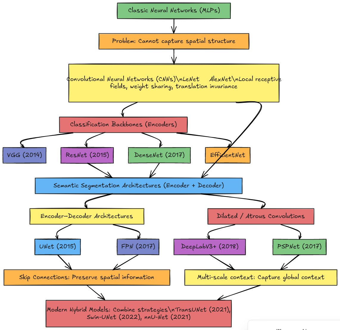
Classic Neural Networks (MLPs) form the foundation of deep learning. These fully connected networks treat images as flat vectors—a 256×256 image becomes a 65,536-element vector. While theoretically capable of learning any function, MLPs cannot capture spatial structure: they don’t understand that adjacent pixels are related or that an edge in one location is fundamentally the same pattern as an edge elsewhere.

Convolutional Neural Networks (CNNs), pioneered by LeNet (1998) and popularized by AlexNet (2012), addressed this limitation through three key innovations: local receptive fields (each neuron sees only a small image region), weight sharing (the same filter applies across the entire image), and translation invariance (a pattern is recognized regardless of position). These principles enabled the hierarchical feature learning that makes modern computer vision possible.

The CNN paradigm then branched into two directions. Classification backbones (also called encoders) like VGG (2014), ResNet (2015), DenseNet (2017), and EfficientNet focus on compressing images into compact feature representations for tasks like “Is this a cat or a dog?” These architectures progressively reduce spatial dimensions while increasing feature channels, culminating in a feature vector that summarizes the entire image.

Semantic segmentation architectures require a different approach: rather than a single label per image, they must produce a label for every pixel. This necessitates encoder-decoder designs that first compress the image (encoding) and then expand it back to full resolution (decoding). Two major families emerged:

1. Encoder-Decoder Architectures like U-NET (2015) and FPN (2017) use skip connections to preserve spatial information lost during encoding. U-NET’s symmetric design with concatenation-based skip connections became the standard for biomedical image segmentation, while FPN’s addition-based lateral connections excel at detecting objects of varying sizes.

2. Dilated/Atrous Convolution Architectures like DeepLabV3+ (2018) and PSPNet (2017) take a different approach: instead of aggressive downsampling, they use dilated convolutions to capture multi-scale context while maintaining spatial resolution. These architectures excel at capturing global context—understanding that a pixel belongs to a cell requires understanding the surrounding tissue structure.

Modern hybrid models like TransUNet (2021), Swin-UNet (2022), and nnU-Net (2021) combine strategies from both families, often incorporating attention mechanisms from transformer architectures to further improve segmentation quality.

For our urothelial cell segmentation task, we focus on the encoder-decoder family, specifically U-NET with ResNet34 as the encoder backbone—combining the proven feature extraction capabilities of residual networks with U-NET’s precise localization through skip connections.

10.2 Part 1: Foundations of Convolutional Neural Networks

10.2.1 9.1 Why Convolution?

The fully connected networks of chapter 9 treat images as flat vectors, losing all spatial information. Consider an image as a tensor where adjacent pixels often encode related information about edges, textures, and shapes. Convolution exploits this locality by applying small filters (kernels) across the image, detecting local patterns. This approach reduces parameters through weight sharing—the same filter is applied across the entire image—making networks more efficient and more adept at capturing spatial hierarchies.

The convolution operation itself is familiar from classical image processing. When applied in neural networks, however, convolution becomes learnable: the network optimizes filter weights through backpropagation to detect patterns most relevant to the task. Beyond convolution, pooling layers aggregate information across spatial regions, providing translational invariance and dimensionality reduction. These operations create a hierarchy where early layers detect simple features (edges, corners) and deeper layers detect increasingly complex, abstract features (eyes, wheels, cells).

10.2.2 9.2 The Convolution Operation

Convolution is the fundamental operation that gives CNNs their name and their power. In the context of neural networks, convolution involves sliding a small learnable filter (also called a kernel) across an input image, computing element-wise multiplications and summing the results at each position.

Figure 10.2: Convolution and Pooling Operations

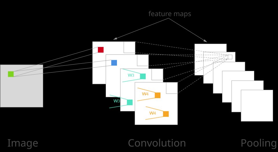
How Convolution Works:

Consider a 3×3 filter sliding across an image. At each position, the filter overlaps with a 3×3 region of the image. The nine corresponding pixel values are multiplied by the nine filter weights, and these products are summed to produce a single output value. The filter then shifts (typically by one pixel, called stride=1) to the next position, and the process repeats. The collection of all output values forms a feature map.

A CNN layer typically applies multiple filters simultaneously—each filter learns to detect a different pattern. For example, one filter might detect horizontal edges, another vertical edges, and another diagonal edges. The outputs from all filters are stacked along the channel dimension, producing a multi-channel feature map.

Key Parameters:

• Filter size: Common choices are 3×3, 5×5, or 7×7. Smaller filters are computationally efficient and can be stacked to achieve larger effective receptive fields.
• Stride: The step size between filter applications. Stride=1 preserves spatial dimensions; stride=2 halves them.
• Padding: Adding zeros around the image boundary to control output size. “Same” padding preserves input dimensions; “valid” padding (no padding) reduces them.
• Number of filters: Determines the number of output channels and thus the richness of learned features.

What Convolution Learns:

In early layers, filters often learn patterns resembling classical image processing operators: - Edge detectors similar to Sobel filters - Blob detectors similar to Laplacian of Gaussian - Oriented patterns similar to Gabor filters

However, these filters are optimized for the specific task through training, not hand-designed. Deeper layers combine these simple patterns into increasingly complex features—corners, textures, object parts, and eventually whole objects or structures like cell nuclei.

10.2.3 9.3 Pooling Operations

Pooling layers reduce the spatial dimensions of feature maps while retaining important information. The two most common pooling operations are:

Max Pooling: Takes the maximum value within each pooling window. A 2×2 max pooling with stride 2 reduces each spatial dimension by half, keeping only the strongest activation in each region. This provides: - Dimensionality reduction (fewer parameters in subsequent layers) - Translation invariance (small shifts don’t change the output) - Noise reduction (weak activations are discarded)

Average Pooling: Takes the mean value within each pooling window. This provides smoother downsampling but may blur strong features.

The Trade-off: Pooling discards spatial information. While this is acceptable for classification (we only need to know “there is a nucleus somewhere”), it becomes problematic for segmentation where we need precise pixel-level predictions. This is why architectures like U-NET use skip connections to recover lost spatial detail.

10.2.4 9.4 Core Components of CNN Architectures

Convolutional layers form the foundation of CNN architectures. A convolutional layer applies multiple learnable filters to the input, each filter producing a feature map. The filter size, stride (step size between filter applications), and padding (whether to extend the image boundary) are design parameters that affect output dimensions and computational cost. By stacking convolutional layers, the network builds increasingly abstract representations while reducing spatial dimensions.

Pooling layers, typically max pooling or average pooling, downsample feature maps by taking the maximum or average value within local windows. Pooling reduces spatial dimensions, decreases parameters, and provides some invariance to small translations. However, aggressive pooling discards detailed spatial information, which becomes problematic when precise pixel-level predictions are required.

Activation functions (ReLU, leaky ReLU, etc.) introduce non-linearity, enabling the network to learn non-linear relationships between features. Normalization techniques such as batch normalization stabilize training by normalizing layer inputs, reducing internal covariate shift and allowing higher learning rates.

Skip connections or residual connections allow information to bypass layers, addressing the vanishing gradient problem in deep networks and facilitating training of very deep architectures.

10.2.5 9.5 Fully Convolutional Networks (FCNs): The Key to Segmentation

To perform image segmentation—producing a class label for every pixel—we need a fundamental architectural change from classification networks. This is where Fully Convolutional Networks (FCNs) become essential.

The Problem with Classification Networks:

Traditional classification CNNs like AlexNet or the original VGG end with fully connected (dense) layers. These layers require a fixed-size input and produce a single output vector (class probabilities). The fully connected layers destroy spatial information:

• A 256×256 image is compressed through convolutions to, say, 8×8×512
• This is then flattened to a 32,768-element vector
• Fully connected layers map this to class scores (e.g., 1000 classes for ImageNet)

The flattening step is the problem: once we flatten, we lose all spatial structure. We can no longer ask “where in the image is the nucleus?” only “is there a nucleus somewhere?”

The FCN Solution:

A Fully Convolutional Network contains only convolutional layers—no fully connected layers anywhere. This simple change has profound implications:

1. Spatial information is preserved: The output is a feature map, not a vector. Each spatial location in the output corresponds to a region in the input.

2. Any input size works: Without fully connected layers (which require fixed dimensions), the network can process images of arbitrary size.

3. Per-pixel predictions: By upsampling the output feature maps back to the input resolution, we obtain a prediction for every pixel.

The seminal FCN paper by Long, Shelhamer, and Darrell (2015), titled “Fully Convolutional Networks for Semantic Segmentation,” demonstrated that classification networks could be converted to FCNs by replacing fully connected layers with convolutional layers, then adding upsampling to recover spatial resolution.

Classification CNN vs. FCN:

Aspect	Classification CNN	Fully Convolutional Network
Final layers	Fully connected	Convolutional
Output	Single label per image	Label per pixel
Input size	Fixed (e.g., 224×224)	Any size
Spatial info	Lost at flatten step	Preserved throughout
Use case	“Is this a cat?”	“Which pixels are cat?”

All Segmentation Architectures are FCNs:

Segmentation Architecture Encoder Backbone (model_key) (encoder_name) ───────────────────── ────────────────── Unet × ResNet18 FPN × ResNet34 DeepLabV3+ × ResNet50 Linknet × EfficientNet-B0 PSPNet × VGG16 MAnet × MobileNet-V2 … × …

Every modern segmentation architecture—U-NET, FPN, DeepLabV3+, PSPNet—is fully convolutional. They differ in how they:

• Encode: How they compress the image into feature representations (the encoder/backbone)
• Decode: How they upsample back to full resolution (the decoder)
• Connect: How they pass information between encoder and decoder (skip connections)

The segmentation_models_pytorch library supports over 400 encoder backbones. The major families include:

ResNet: resnet18, resnet34, resnet50, resnet101, resnet152 EfficientNet: efficientnet-b0 through efficientnet-b7 VGG: vgg11, vgg13, vgg16, vgg19 (with or without batch norm) DenseNet: densenet121, densenet161, densenet169, densenet201 MobileNet: mobilenet_v2, timm-mobilenetv3_large Inception, Xception, DPN, SE-ResNet, and many more

But they all share the FCN principle: no fully connected layers, spatial information preserved, per-pixel output.

Converting Classification Networks to FCN Encoders:

Classification networks like ResNet34 can serve as FCN encoders by simply removing the final fully connected layers:

• Original ResNet34: Conv layers → Global Average Pooling → FC layer → 1000 class scores
• ResNet34 as FCN encoder: Conv layers → Stop here, output feature maps to decoder

This is exactly what happens when we use encoder_name="resnet34" in our segmentation model—the classification head is removed, and the convolutional backbone becomes part of a fully convolutional segmentation network.

Why This Matters for Our Project:

For urothelial cell segmentation, we need to identify the exact pixels belonging to nucleus, cytoplasm, and background. This is impossible with a classification network that outputs only “this image contains a cell.” We need an FCN that outputs a 256×256×3 prediction map, where each of the 65,536 pixels receives its own class prediction.

Our model (FPN with ResNet34 encoder) is fully convolutional:

• ResNet34 encoder: All convolutional layers (FC layers removed)
• FPN decoder: Lateral connections (1×1 convolutions) + upsampling + convolutions
• Output: 1×1 convolution producing per-pixel class scores

No fully connected layers anywhere—this is what enables pixel-level segmentation.

10.3 Part 2: ResNet Architecture—Learning with Residual Connections

10.3.1 9.6 The Problem of Depth

As researchers attempted to build deeper networks in the early 2010s, they encountered a paradox: adding more layers should increase representational power, yet very deep networks (20+ layers) often performed worse than shallower ones. This wasn’t due to overfitting—even training error increased with depth.

The culprit was the vanishing gradient problem. During backpropagation, gradients must flow backward through every layer. With each layer, gradients can shrink (vanish) or explode, making it difficult to update weights in early layers effectively. By the time gradients reach the first few layers of a 50-layer network, they may be too small to drive meaningful learning.

10.3.2 9.7 The Residual Learning Solution

ResNet (Residual Network), introduced by He et al. in 2015, solved this problem with a remarkably simple idea: residual connections (also called skip connections or shortcut connections).

Figure 10.3: ResNet34 Architecture

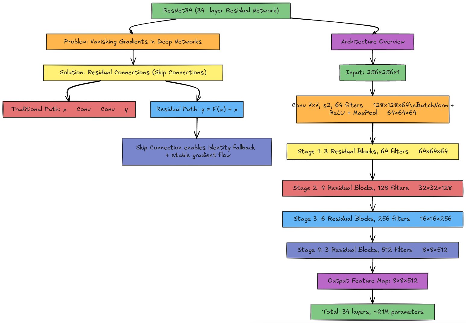
Instead of learning the direct mapping from input to output, each block learns the residual—the difference between the desired output and the input:

Traditional block: \[y = F(x)\]

Residual block: \[y = F(x) + x\]

Here, \(F(x)\) represents the transformations within the block (convolutions, batch normalization, ReLU), and \(x\) is the input passed directly through the skip connection.

Why Residuals Work:

1. Identity mapping as baseline: If \(F(x)\) learns nothing useful (outputs zeros), the block simply passes through \(x\) unchanged. The network can never do worse than the identity function.

2. Gradient flow: During backpropagation, gradients flow directly through the skip connection, bypassing the nonlinear layers. This creates an unimpeded “gradient highway” that enables training of very deep networks.

3. Easier optimization: Learning small residual adjustments is often easier than learning complete transformations from scratch.

10.3.3 9.8 ResNet34 Architecture

ResNet34, with 34 weighted layers, represents a practical balance between depth and computational cost. It is commonly used as an encoder backbone in segmentation architectures like U-NET and FPN.

Overall Structure:

ResNet34 consists of:

1. Initial convolution: A 7×7 convolution with stride 2 and 64 filters, followed by batch normalization, ReLU, and 3×3 max pooling. This rapidly reduces spatial dimensions from 256×256 to 64×64 (for a 256×256 input).

2. Four stages of residual blocks:

   • Stage 1: 3 residual blocks, 64 filters each → Output: 64×64×64
   • Stage 2: 4 residual blocks, 128 filters each → Output: 32×32×128
   • Stage 3: 6 residual blocks, 256 filters each → Output: 16×16×256
   • Stage 4: 3 residual blocks, 512 filters each → Output: 8×8×512

3. Classification head (for standalone use): Global average pooling followed by a fully connected layer. For segmentation, this head is removed and replaced with a decoder.

The Basic Residual Block:

Each basic block in ResNet34 contains:

Input (x)
    │
    ├──────────────────────┐
    ↓                      │
3×3 Conv, BatchNorm, ReLU  │ (skip connection)
    ↓                      │
3×3 Conv, BatchNorm        │
    ↓                      │
    + ←────────────────────┘
    ↓
   ReLU
    ↓
Output (y = F(x) + x)

When the number of channels changes between stages (e.g., from 64 to 128), a 1×1 convolution is applied to the skip connection to match dimensions.

10.3.4 9.9 Why ResNet34 for Cell Segmentation?

ResNet34 offers several advantages as an encoder for urothelial cell segmentation:

1. Proven feature extraction: Pre-trained on ImageNet’s 1.2 million images, ResNet34 has learned robust low-level features (edges, textures) that transfer well to microscopy images.

2. Appropriate depth: Deep enough to capture complex cell morphology, yet not so deep as to require excessive computation or risk overfitting on limited biomedical datasets.

3. Multi-scale features: The five stages produce feature maps at different resolutions (256, 64, 32, 16, 8 pixels for a 256×256 input), which U-NET’s decoder can use via skip connections.

4. Computational efficiency: With ~21 million parameters, ResNet34 is manageable for training on single GPUs, unlike larger variants like ResNet101 or ResNet152.

10.3.5 9.10 Connecting ResNet to Segmentation

When used as an encoder in U-NET or FPN, ResNet34 is modified:

1. Remove the classification head: The global average pooling and fully connected layers are discarded.

2. Extract intermediate features: Feature maps from each stage are tapped for skip connections:

   • Stage 1 output (64×64×64): Fine spatial detail
   • Stage 2 output (32×32×128): Local patterns
   • Stage 3 output (16×16×256): Cell-level features
   • Stage 4 output (8×8×512): Semantic context

3. Feed to decoder: The decoder upsamples from 8×8 back to 256×256, concatenating (U-NET) or adding (FPN) features from corresponding encoder stages at each resolution.

This combination—ResNet’s powerful feature extraction with U-NET’s precise localization—forms the backbone of our cell segmentation pipeline.

10.4 Part 3: U-NET Architecture and Principles

10.4.1 9.11 The U-NET Architecture

U-NET, introduced by Ronneberger, Fischer, and Brox (2015), is a fully convolutional network designed specifically for biomedical image segmentation. Its distinctive architecture resembles a “U” shape: a contracting (encoder) path followed by an expanding (decoder) path, with skip connections linking corresponding encoder and decoder levels.

The contracting path applies repeated convolution and max-pooling operations, progressively downsampling the image and increasing the number of feature channels. Each downsampling step is a block consisting of two 3×3 convolutional layers (followed by ReLU) and one 2×2 max-pooling operation, halving spatial dimensions and doubling channels.

The bottom of the U consists of convolutional layers at the lowest spatial resolution, capturing the most abstract features.

The expanding path upsamples feature maps using either transpose convolutions (deconvolutions) or interpolation followed by convolution. Each upsampling step increases spatial dimensions and typically reduces channels. Critically, skip connections concatenate feature maps from the corresponding encoder level to each decoder level. These skip connections provide the decoder with fine-grained spatial information from early encoder layers, enabling precise localization in the output segmentation.

The final layer is a 1×1 convolution that maps the feature maps to the desired number of output classes, producing the segmentation map.

10.4.2 9.12 Skip Connections and Information Flow

Skip connections are central to U-NET’s success. During the encoding path, spatial detail is progressively lost as the resolution decreases. The decoder pathway must reconstruct this detail to make accurate pixel-level predictions. Skip connections alleviate this by directly passing high-resolution feature maps from the encoder to the decoder, bypassing the intermediate layers.

When a decoder level is upsampled to match the spatial resolution of a corresponding encoder level, the upsampled features are concatenated (channel-wise) with the encoder features. This concatenation allows the decoder to access both the fine-grained spatial information from the encoder and the semantic information accumulated in deeper layers, striking a balance between localization and semantic understanding.

This design principle—combining low-level spatial detail with high-level semantic context—is fundamental to U-NET’s effectiveness for segmentation tasks requiring precise boundaries, such as cell segmentation in microscopy images.

10.4.3 9.13 Loss Functions and Metrics for Segmentation

Unlike classification, where a single prediction per image is evaluated, segmentation produces predictions for every pixel. Cross-entropy loss, computed per pixel and averaged, remains common. However, medical image segmentation often employs specialized loss functions.

The Dice loss (F1 loss) is a region-based loss measuring the overlap between predicted and true segmentation regions. It is particularly useful when classes are imbalanced (e.g., if foreground objects occupy only a small fraction of the image). The Dice coefficient is 2 times the intersection divided by the sum of the two sets’ sizes.

Focal loss addresses class imbalance by down-weighting easy (well-classified) pixels and focusing training on hard examples.

IoU (Intersection over Union) measures the overlap between predicted and true regions as the ratio of intersection to union. It is more stringent than pixel accuracy, penalizing even small boundary misalignments.

The Dice coefficient, similar to IoU but slightly different mathematically, is widely used as both a loss function and an evaluation metric in biomedical segmentation.

10.5 Part 4: Application to Urothelial Cell Segmentation

10.5.1 9.14 The Urothelial Cell Dataset

Urothelial cells, the epithelial cells lining the urothra and bladder, are important in clinical diagnostics and research. Microscopy images of urothelial cell cultures or tissue samples are often accompanied by manual or semi-automated annotations delineating cell boundaries, nuclei, or other structures of interest. The dataset for our case study consists of (briefly describe: grayscale or multi-channel microscopy images, image resolution, number of samples, annotation format).

The segmentation task is to identify and delineate individual cell boundaries or nuclei boundaries, producing a binary mask (cell/non-cell) or multi-class mask (cell nuclei, cytoplasm, background, etc.), depending on the research objective.

This dataset is chosen not only because of its biological relevance but also because it exemplifies challenges common in biomedical image analysis: limited sample sizes (typically tens to hundreds of images), high annotation cost (manual labeling by experts), spatial variations (cell size, shape, and morphology vary), and the need for precise boundary delineation.

10.5.2 9.15 Data Preparation and Augmentation for Urothelial Cells

The raw urothelial cell images and corresponding annotation masks are loaded from the dataset repository. Images may be grayscale (single channel) or fluorescent multi-channel acquisitions. If multi-channel, images may be converted to grayscale, kept as separate channels, or fused into a composite. Masks are typically binary (foreground/background) or multi-class (nucleus, cytoplasm, background).

Preprocessing includes normalization of image intensity to [0, 1] or standardization using the training set mean and standard deviation. Masks are converted to integer class labels and one-hot encoded if necessary.

Given the limited size of typical microscopy datasets, data augmentation is crucial. Rotation, horizontal and vertical flips, small translations, and elastic deformations are applied randomly to training images and corresponding masks, artificially increasing dataset diversity and improving the model’s robustness to variations in cell orientation and positioning.

Images and masks may be cropped into smaller tiles (e.g., 256×256 or 512×512 pixels) to fit into memory and to provide more training samples from a single large image.

10.5.3 9.16 Model Configuration and Training Strategy

The U-NET model is instantiated with specific hyperparameters: initial number of filters (e.g., 64), depth (number of levels in the U, e.g., 5 levels), and whether to use batch normalization, dropout, or other regularization techniques.

The model is compiled with an optimizer (Adam is standard), a loss function (binary cross-entropy for binary segmentation, categorical cross-entropy for multi-class, or Dice loss for region-aware learning), and metrics (pixel accuracy, Dice coefficient, IoU).

Training uses the train-validation-test split prepared earlier. During training, the model processes batches of images and masks, computes loss across all pixels, and updates weights via backpropagation. A validation set is evaluated after each epoch to monitor overfitting and to enable early stopping (halting training if validation loss ceases to improve).

Due to limited data, regularization techniques such as dropout, data augmentation, and possibly transfer learning (initializing weights from a model trained on a larger dataset) may be employed to prevent overfitting.

10.5.4 9.17 Evaluation on Urothelial Cell Segmentation

After training, the model is evaluated on a held-out test set. Quantitative metrics include per-class Dice coefficient, IoU, and pixel accuracy. Qualitative evaluation involves visual inspection of predicted segmentation maps overlaid on original images, identifying successes and failure modes (e.g., touching cells merged into a single region, small cells missed, boundary imprecision).

Error analysis may reveal patterns: Do segmentation errors occur more frequently in regions with certain characteristics (e.g., crowded cells, low contrast, cell boundaries)? Such insights guide architectural modifications or additional data collection strategies.

The model’s predictions can be post-processed: morphological operations (opening, closing) can clean up noisy predictions; connected component analysis can separate touching cells if the goal is instance segmentation (identifying individual cell instances, not just class membership).

10.5.5 9.18 Deployment and Practical Considerations

Once validated, the trained U-NET can be deployed to segment new, unseen microscopy images from the same institution and microscope setup. However, domain shift—differences in image acquisition (microscope, staining protocol, imaging parameters)—can degrade performance. Fine-tuning on a small set of images from the new domain often recovers performance.

Computational efficiency is relevant: U-NET is memory-intensive due to stored activations in skip connections. Inference (forward pass without gradient computation) is faster than training but may still require acceleration via GPU or model quantization if real-time or near-real-time processing is required.

The trained model can serve a variety of downstream applications: automated cell counting, morphological analysis, identifying cellular phenotypes, or flagging anomalies for expert review in a clinical or research pipeline.

10.6 Part 5: Extensions and Advanced Topics

10.6.1 9.19 Variants and Extensions of U-NET

U-NET has spawned numerous variants addressing specific challenges and datasets. Attention U-NET incorporates attention mechanisms that learn which spatial regions or channels are most relevant for segmentation, potentially improving performance on imbalanced or complex datasets. 3D U-NET extends the 2D architecture to volumetric data (e.g., CT, MRI, confocal microscopy stacks), using 3D convolutions and pooling operations.

Recurrent U-NET incorporates recurrent connections to model temporal dynamics, useful for segmenting video or time-lapse microscopy. Dense U-NET uses dense connections (concatenating all previous layers) inspired by DenseNet, potentially improving feature propagation and reducing parameters.

10.6.2 9.20 Multi-task and Transfer Learning with U-NET

U-NET is flexible and can be adapted for multi-task learning: jointly training on segmentation and another related task (e.g., cell type classification, boundary detection). The shared encoder learns representations useful for both tasks, potentially improving generalization.

Transfer learning leverages models trained on large datasets. A U-NET pre-trained on a large microscopy dataset can be fine-tuned on the specific urothelial cell dataset with fewer training iterations, reducing training time and improving final performance when training data is limited.

10.6.3 9.21 Instance Segmentation and Post-processing

Semantic segmentation, as presented, assigns a class to each pixel but does not distinguish between instances. If the goal is instance segmentation (separating individual cells even if they are of the same class), post-processing is needed. Connected component analysis identifies separate connected regions. Watershed segmentation refines boundaries between touching instances. More sophisticated approaches train models to predict boundaries or distance maps, facilitating instance separation.

10.6.4 9.22 Challenges and Limitations

U-NET and segmentation in general face challenges. Class imbalance (if foreground is rare) biases training toward background. Limited training data risks overfitting, particularly in high-dimensional networks. Boundary precision can be sensitive to preprocessing and hyperparameters. Domain shift (distributional differences between training and deployment data) often requires fine-tuning or domain adaptation techniques.

Annotation cost is prohibitive for large datasets, motivating research into semi-supervised and self-supervised learning approaches that leverage unlabeled data.

10.7 Summary and Transition

In this chapter, we have explored convolutional neural networks and U-NET, understanding how convolutional layers and skip connections enable precise pixel-level segmentation. We examined the evolution from classic neural networks through CNNs to modern segmentation architectures, and studied ResNet34’s residual learning approach that enables training of deep networks. We then turned to a real-world application: segmenting urothelial cells in microscopy images, navigating data preparation, model design, training, and evaluation.

Segmentation is a powerful tool for automated image analysis. U-NET’s effectiveness and relative simplicity have made it a standard in biomedical image processing. However, it is one of many architectures; emerging approaches such as Transformers, self-supervised models, and hybrid architectures continue to expand the landscape. In subsequent chapters, we may explore these frontiers, or expand into related domains such as object detection and instance segmentation, where the goal is both localizing and classifying distinct entities within images.

The principles learned here—layer-wise feature extraction, residual connections, skip connections, pixel-wise loss computation, data augmentation, and careful validation—extend beyond U-NET to a broad class of deep learning architectures and applications.

---

10.8 Notes for Development

Conceptual Level: This draft is organized by pedagogical progression, beginning with foundational concepts (neural network architecture overview, why convolution is useful), introducing encoder architectures (ResNet34), presenting the segmentation architecture (U-NET), and finally applying it to a realistic dataset (urothelial cells).

Code Placement: As requested, no code is included in this draft. Code would be placed in subsections or appendices, showing instantiation of models, training loops, and evaluation routines.

Figures Required:

• images/nn_architecture_flowchart.png: Neural network architecture evolution diagram
• images/convolution_pooling.png: Convolution and pooling operations illustration
• images/resnet34_architecture.png: ResNet34 architecture diagram

Exercises: Opportunities for student exercises include: - Tracing the dimensions through a ResNet34 encoder for different input sizes - Implementing a custom loss function combining cross-entropy and Dice loss - Designing and experimenting with U-NET variants (adding attention, dropout, etc.) - Analyzing failure modes in urothelial cell segmentation and proposing remedies - Comparing segmentation results with different encoder backbones (ResNet18 vs ResNet34 vs ResNet50)

Figures and Visualizations: The chapter would benefit from figures illustrating: - Neural network architecture family tree (included) - Convolution operation and filter sliding across an image (included) - ResNet34 architecture with residual blocks (included) - U-NET architecture diagram with skip connections explicitly labeled - Urothelial cell raw images, ground-truth masks, and model predictions - Metrics (Dice, IoU) visualized as the network trains

Grading and Assessment Tools: For your automated grading system, consider: - Programmatic verification that students correctly load and preprocess the dataset - Tests ensuring the model architecture matches specifications (layer types, skip connection placement, output dimensions) - Metrics computation to verify students correctly implement Dice coefficient or IoU calculations - Visualization generation (segmentation overlays) for human inspection